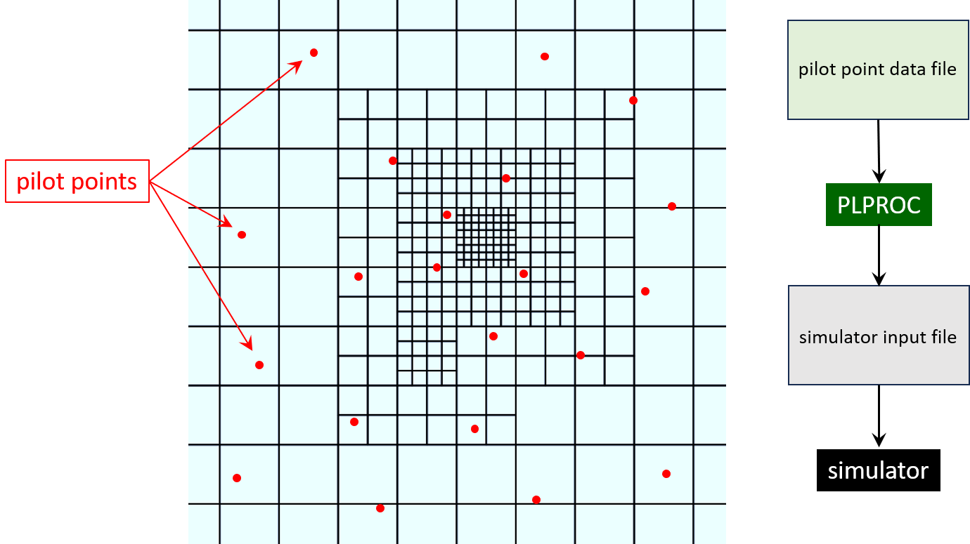
The figure below shows a quadtree-refined model grid, with an irregular array of pilot points spread throughout the model domain.

In the simplest deployment of pilot points, assignment of hydraulic properties to cells of a model grid is a two-step process. First, hydraulic property values are assigned to pilot points. Then these values are spatially interpolated to the centres of model grid cells.

This operation implies that a preprocessor runs before the simulator, this preprocessor being part of the model sandwich that is run by PEST. This preprocessor is normally PLPROC. PLPROC reads a file which contains hydraulic property values that are assigned to pilot points. It interpolates these values to the cells of a model grid, and then records these interpolated values in a file that the model can read.

Pilot point parameterisation of a model grid.

Actually, use of pilot points can get much more complicated than this. It is your choice.

Pilot points can be used to modify existing model hydraulic properties. Thus the model preprocessor may read an existing model input file. It may then interpolate multipliers that are ascribed to pilot points to an array that is compatible with this existing hydraulic property array. It may then add these two arrays together, or multiply one of them by the other, or perform even more complex operations between them. It then records the modified array in model-ready format.

Perhaps the original model-compatible array was assigned values through spatial interpolation from a broadly-disposed set of pilot points. A second set of pilot points can then be used to add detail to part of the first array. This second set of pilot points may be localised to the part of the array that requires modification. Modification may involve multiplication of the original array, or the performance of some nonlinear operation on it.

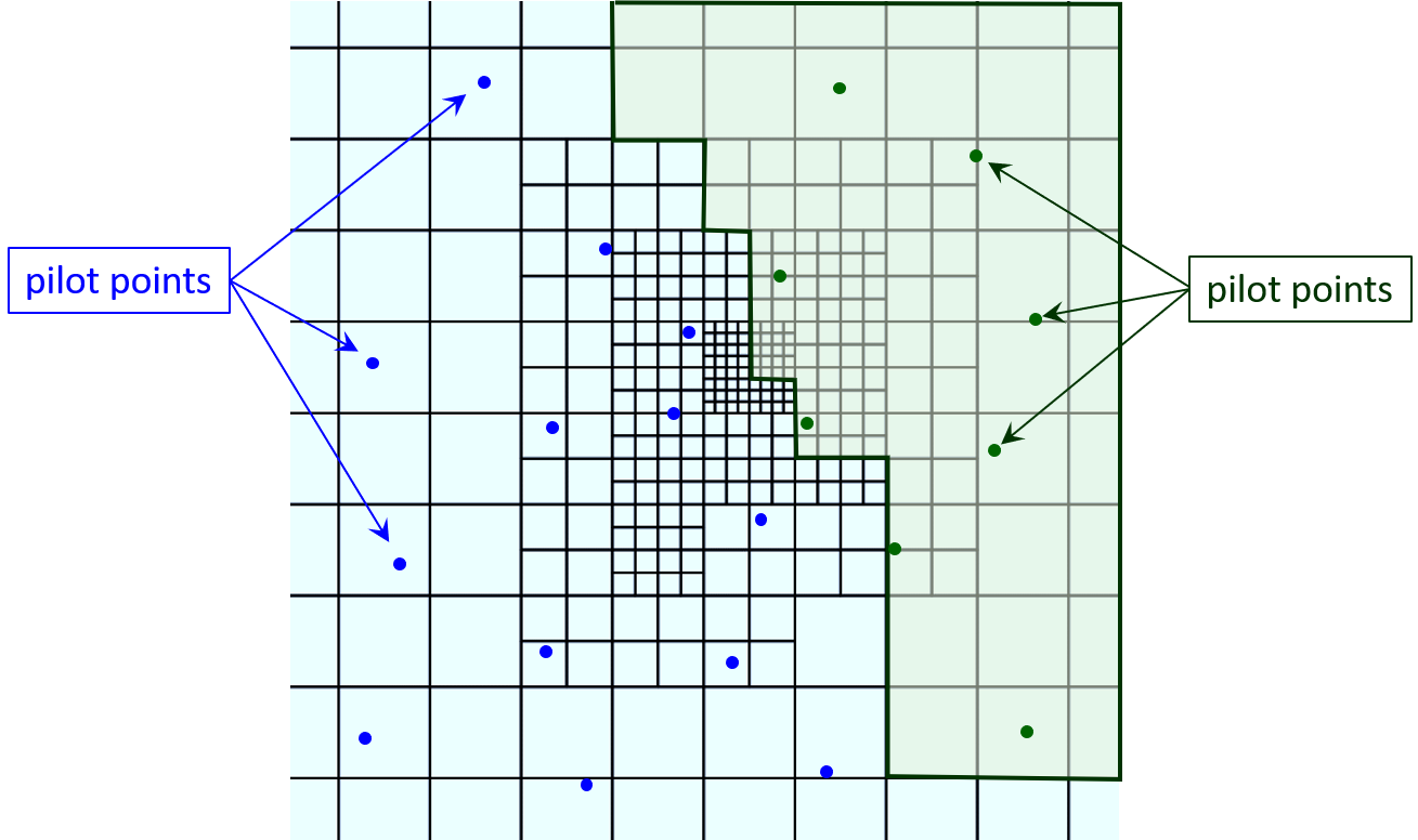
In the figure below the blue pilot points are assigned to the zone on the left, while the green pilot points are assigned to the zone on the right. When different pilot points are assigned to different zones, no spatial interpolation takes place across zone boundaries. Hence hydraulic property discontinuities are maintained at zone boundaries.

Pilot points assigned to different zones.

There is no limit on the creativity that you can exercise in design of a model parameterisation scheme that is based wholly or partly on pilot points. For example, you can use PEST to estimate zone-based hydraulic property values. Pilot point multipliers can then be assigned to these same zones. The pilot points can therefore take care of spatial hydraulic property detail while the zonal values can take care of broad scale hydraulic property parameterisation that may be based on geological mapping

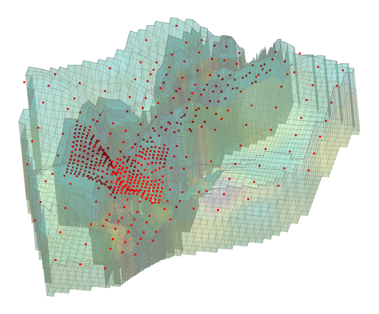
Pilot points can be one-, two- or three-dimensional. In one-dimension they can be used to undertake linear interpolation along polylines. In two dimensions they can be used to assign hydraulic properties to a single model layer. In three dimensions they can be used to assign properties to many model layers. All of these can be combined in a single model.

A multi-layer model that uses two and three-dimensional pilot points.

Interpolation from pilot points to a model grid can employ a variety of interpolation methodologies. Furthermore, interpolation can be isotropic or anisotropic. In special circumstances, anisotropic interpolation can follow the path of an alluvial boundary.

Pilot point parameterisation of an alluvial system.