PLPROC stands for "parameter list processor". Initially, PLPROC was written to facilitate pilot point parameterisation of both structured and unstructured grid models. However over time, its functionality has extended way beyond this.

A "list" is an array of integer or real numbers. A two- or three-dimensional spatial coordinate is associated with each element of the list. Elements can pertain to cells of a model grid, to individual pilot points, or to vertices of a polyline or polygon.

Many of PLPROC's operations support inference of numbers in one list from those of another, mainly through spatial interpolation. Subsets of lists can be selected for processing using logical relationships based on equations of arbitrary complexity. Meanwhile, mathematical operations of arbitrary mathematical complexity can be performed between lists that belong to the same family (i.e. that share the same element coordinates).

User-specified items of PLPROC functionality are invoked through function calls. A PLPROC input file is therefore a type of script file. Each function has many options; these are expressed through its arguments. A PLPROC script of even moderate length can perform model preprocessing operations that have a high level of sophistication. Model parameterisation can therefore be context-sensitive and creative.

PLPROC records the outcomes of its calculations on model input files. Like PEST, it uses template files to transfer numbers to these files in order to ensure a non-intrusive model interface. However PLPROC template files are more sophisticated than those that PEST uses. Whole lists of numbers can be recorded on a model input file using a single "embedded function" that resides in a template file. Embedded functions are also smart enough to select individual elements of a list for recording on a particular line of a model input file; element selection can depend on other information that is stored on the same line of the model input file to which data are being transferred.

Part of a PLPROC script follows. Do not be daunted. PLPROC is well documented. The functions are straightforward to use. Error detection is thorough and informative.

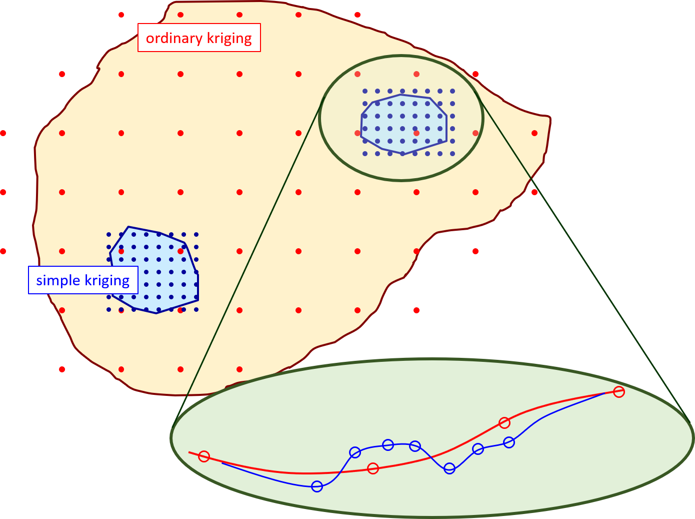
A few PLPROC options are briefly discussed. See the manual for details.

Spatial interpolation

PLPROC supports kriging, radial basis functions and inverse power of distance interpolation in two and three dimensions.  These can respect, or transgress, model zonation boundaries; it is your choice.

Which is the best to use? Kriging is generally best. There are a few reasons for this. They include the following.

•The highest and lowest values of an interpolated hydraulic property field are normally at pilot point locations themselves rather than in between them. This means that parameter bounds that are used in a PEST control file apply to interpolated values, as well as to pilot point parameter values that are adjusted by PEST.

•Kriging is fast, especially with pre-calculated interpolation factors. (PLPROC allows you to do this.)

•Sometimes interpolation using radial basis functions produces parameter fields that look a little "lumpy" (and hence unrealistic).

However kriging has its disadvantages too. They include the following.

•The interpolated parameter field may contain "bulls eyes". Regularisation using a covariance matrix can help prevent this, but sometimes the bulls eyes remain.

•If the search radius employed for kriging calculation is too small, the interpolated parameter field may have artificial discontinuities. It looks like a bad paint job.

•Use of a single variogram over areas where pilot point spatial density varies widely can introduce interpolation artifacts where the local distance between pilot points is much smaller than the range of the variogram.

PLPROC's calc_kriging_factors_auto_2d() function seems to overcome most of these problems.

Kriging can be simple or ordinary. Simple kriging provides a good option for local warping of background values (which may have been interpolated from another set of pilot points using ordinary kriging). This is because, with simple kriging, interpolated values fade back to the user-prescribed mean value as the distance to the nearest pilot point increases. Where pilot points are multipliers, a suitable mean value is 1.0.

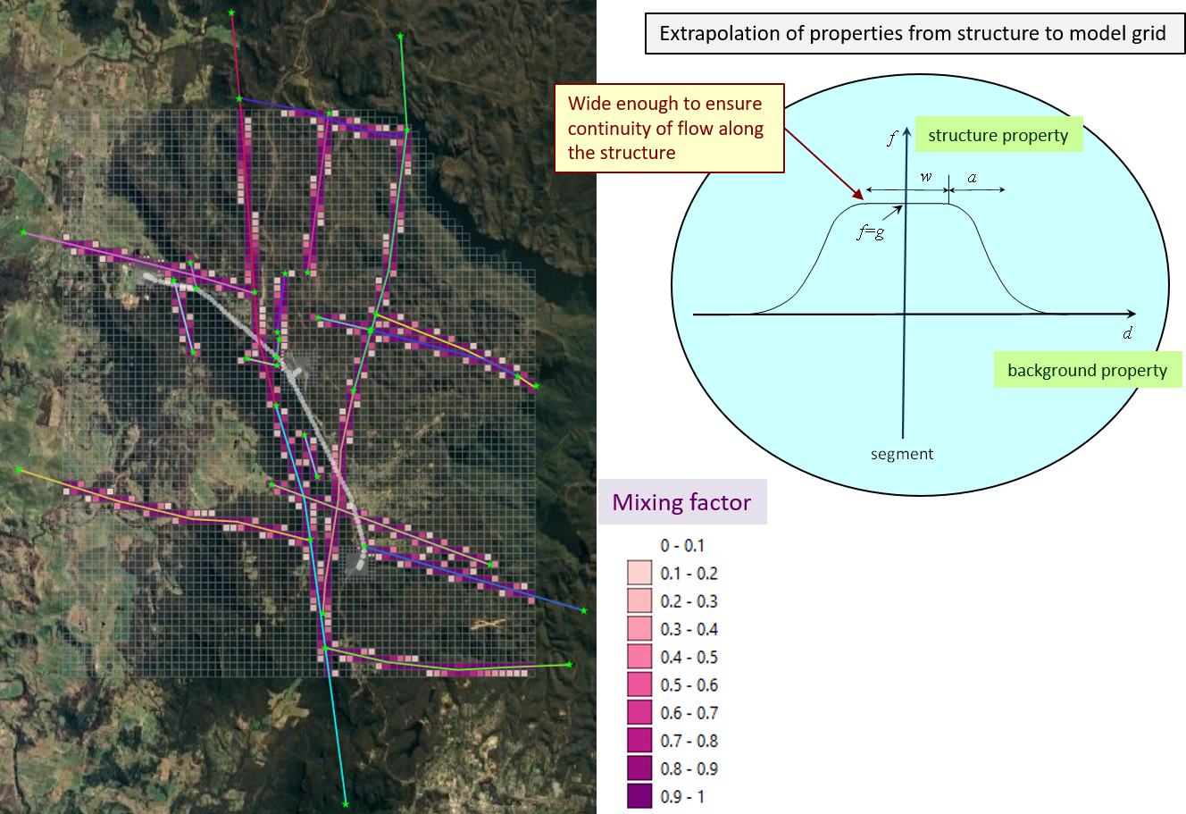
Interpolation functions provided by PLPROC can determine for themselves variogram properties that best support kriging at any location in the model domain, this depending on pilot point spatial density at that location. Meanwhile, the direction and magnitude of anisotropy can vary throughout a model grid in accordance with user specifications, or with the presence (or otherwise) of a nearby alluvial boundary.

Model grid

PLPROC can acquire the coordinates of model grid cell centres by reading grid specification files that are pertinent to different model types, for example structured MODFLOW, MODFLOW-USG and MODFLOW 6. For other models, it can read grid cell centre coordinates from lists contained in tabular or CSV files. PLPROC can record interpolated hydraulic property values to model input files of arbitrary protocol. These protocols may include arrays, lists and tables such as those used by input files for MODFLOW packages such as RIVER, DRAIN, SFR and others.

Hydraulic property mixing

Near structural boundaries, PLPROC can mix properties on one side of the boundary with those on the other side of the boundary. Hence the transition between the two is smooth. This ensures continuity of model outputs with respect to parameter values if some of these parameters can move the boundary.

Using mixing factors along mapped faults.

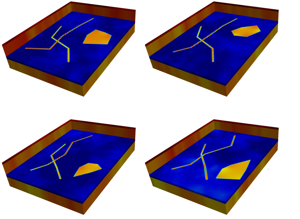
Pilot points can be used to define the vertices of polylines or polygons that describe subsurface geobodies of hydrogeological interest. PLPROC can interpolate hydraulic properties along these lines and within these polygons. At the same time, geobody vertices can move along "sliders" (which can move along other sliders). Faults can therefore change position. Potential holes in an aquitard can change both position and shape. Both the hydraulic properties of these geobodies, and the locations of their vertices can be denoted as model parameters. They can thus be random and/or adjustable, depending on whether you are exploring prior uncertainty or reducing uncertainty through history-matching. Hydraulic properties can change abruptly at geobody boundaries, or blend into background hydraulic properties of host rocks.

Two faults and an aquifer hole. Positions, shapes and hydraulic properties are all history-match-adjustable.

Normally, at least one parameter is associated with each pilot point. In a particular model layer, a set of pilot points may host hydraulic conductivity parameters. They may also host storage parameters, and/or parameters that govern other processes such as subsidence.

PLPROC reads files which provide the locations of pilot points. The same files, or different files, provide values for pilot-point-associated hydraulic properties, or other quantities such as multipliers, that PEST or PEST++ must adjust. A model may play host to thousands of pilot points, and maybe many thousands of pilot point parameters.

This presents us with two tasks. These tasks seem a little complicated at first, but are not as hard as may first appear. They are:

1.Creation of template files of PLPROC input files;

2.Listing of pilot point data in the "parameter data" section of a PEST control file.

Below is the first part of a template file of a PLPROC input file. The first column is for the user's benefit. PLPROC ignores it. Five columns of parameter spaces follow the first column. Each of these spaces contains the name of a parameter that is associated with a particular pilot point. When PEST runs the model, it replaces each of these spaces by the current value of each named parameter. In this particular case, parameters are named after rows and columns of a model grid. This is because pilot point emplacement is regular; in fact, pilot points lie at grid cell centres. A file such as that shown below can be built using a self-written program. However it is not too hard to create it yourself using a spreadsheet.

Adding lots of parameters to the "parameter data" section of a PEST control file can be a little tedious. However if all parameters of the same type have the same initial value, and if all parameters of the same type have the same upper and lower bounds, then this can be done with a little cutting and pasting. Alternatively, help is available from the TPL2PST utility supplied with the PEST suite. If you make any errors, PESTCHEK will find them for you.

Parameters of different types, or that belong to different model layers, should be assigned to different parameter groups. Then, when using ADDREG1 or ADDREG2 to add prior information to the PEST control file for Tikhonov regularisation purposes, these prior information equations will be assigned to different observation groups. This facilitates balancing of weights between them. Remember to keep parameter group names to 6 characters or less if you can. This avoids possible duplication of prior information group names when ADDREG1 or ADDREG adds a "regul_" prefix to the names of parameter groups to form the names of prior information groups.