Use as many pilot points as you can. The more the better. The more that you use, the less do their exact locations matter, and the less does the interpolation method matter.

Some modellers who are new to highly parameterised inversion are a little wary of using lots of pilot points; they fear over-fitting. This is not a problem. Regularisation takes care of uniqueness as it forestalls over-fitting. The more pilot point parameters that you use, the more likely it is that at least some of them are where they need to be to express the heterogeneity that the calibration dataset may require. If pilot points are not in the right place, then pilot points that are in the wrong place will try to do the job. Predictive bias (and possibly "bulls eyes" around certain pilot points) may result.

When doing uncertainty analysis, there must be enough pilot points to express the potential heterogeneity to which predictions of management interest may be sensitive.

Don't forget - calibration is designed to express the heterogeneity that MUST exist to explain measured data. Uncertainty analysis is designed to express the heterogeneity that MAY exist that is compatible with measured data. The more pilot points that you use, the better can both of these jobs be done. Furthermore, failure (through parameter insufficiency) to allow probabilistic expression of prediction-pertinent heterogeneity may diminish the calculated width of predictive uncertainty intervals. Decision-support modelling failure follows.

It is only practical considerations that limit the number of pilot points that you use. Filling of a Jacobian matrix costs at least one model run per iteration of the inversion process. Then, once it has been filled, if the Jacobian matrix is too large, it may be difficult to store and manipulate this matrix. Neither of these is a problem if using ensemble methods, regardless of the number of pilot points in use.

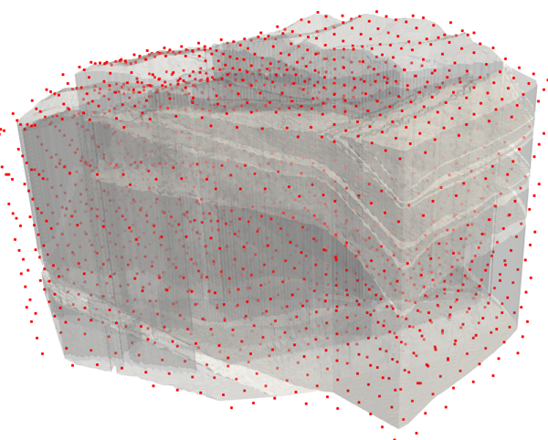
If you are working to a pilot points budget, then strategic (and therefore irregular) placement of pilot points is probably the best option. However if you are using ensemble methods, then perhaps reasonably dense placement of pilot points on a regular grid is a good option (particularly if working in three dimensions).

Pilot points disposed on a regular 3D grid.

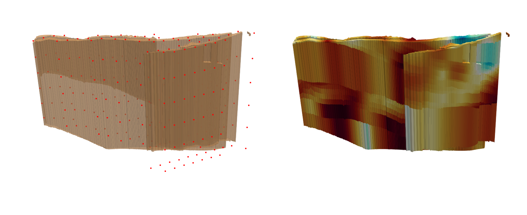
3D emplacement of pilot points along, and near, a structural feature.

It is really important to note that pilot points do not need be confined to inside the area or volume that they inform through interpolation. Sometimes it makes sense for the last row or column of pilot points to be just outside the boundary of a model domain.

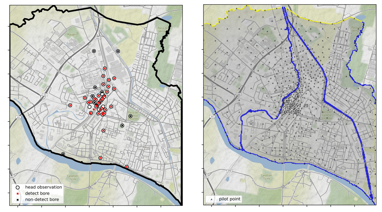
The following approach seems to work well when working in a two-dimensional model domain (for example if assigning pilot points to an individual model layer). It results in a greater density of pilot points where there is a greater density of information. This makes sense. Don't forget that parameters are receptacles for information. They need to be placed where they can most effectively receive information that is resident in a history-matching dataset without distorting that information.

1.First tell yourself how many pilot points that you want to assign to the model layer, and then try to stick to it. (This is normally determined by your computing budget.)

2.Place pilot points between observation wells in the direction of the hydraulic gradient. It is the hydraulic conductivity between wells that determines the head difference between them.

3.Ensure that pilot points are placed between outflow boundaries and the first upstream head measurement wells. Heads in these wells reflect boundary conductances, and the hydraulic conductivity of material between them and the boundary.

4.Place pilot points near the sites of predictions of management interest.

5.Ensure a minimum spatial density of pilot points elsewhere in the model layer.

6.Avoid extrapolation. Place pilot points at model boundaries rather than extrapolating to boundaries. Regularisation will take care of keeping parameter values sensible in places where there is little information. Spatial extrapolation is a more difficult process to tame.

A greater density of pilot points is warranted where there is a greater density of information.