|
<< Click to Display Table of Contents >> Observations |
  
|
|
<< Click to Display Table of Contents >> Observations |
|
Whether or not you work with MODFLOW, there is a lot to be gained by storing field data in a simple file type that is referred to as a "site sample file" or "bore sample file" in PEST parlance. Part of a site sample file follows.
The protocol is simple. •site names are 20 characters or less in length; •date protocols can be dd/mm/yyyy or mm/dd/yyyy; •all entries for one site must follow those for another; •for any site, entries must be supplied in order of time. The SMPCHEK utility supplied with the groundwater utilities can check that a site sample file adheres to all of these protocols. |
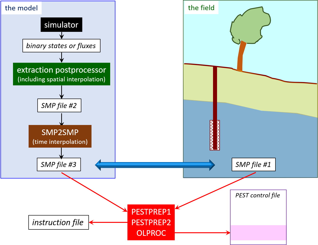
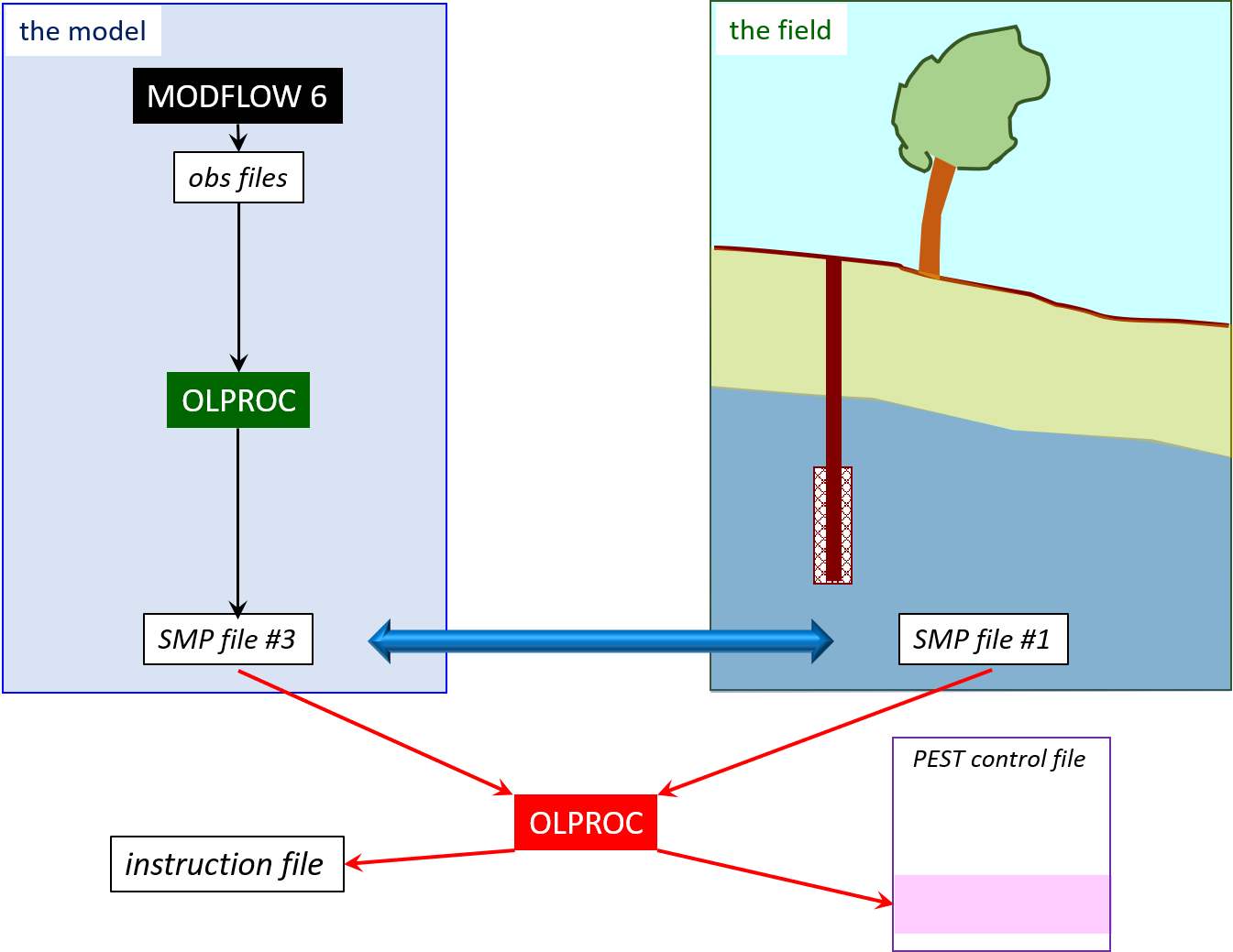
The figure below schematises how model-generated counterparts to field measurements can be extracted from model output files and compared with these field measurements. It also shows how a PEST input dataset can be constructed or modified to include new observations. First look at site sample file #1. This contains field measurements that will be used for model history-matching. Now look at the simulator. If this is a member of the MODFLOW family, it records the system states and fluxes that it calculates in large binary files. Postprocessors must read these files. One postprocessor may collect flux terms over boundary segments where field measurements of flux exist. Another may undertake spatial interpolation from the model grid to the sites at which measurements of system state (for example heads or concentrations) were made. The site-specific, model-generated time series that these model postprocessors produce are recorded in site sample files. Site sample file #2 shown on the left of the above figure is such a file. MODFLOW postprocessors that perform the tasks that are represented by the green box are discussed below. The next step is to implement time-interpolation from the times at which model outputs are recorded in site sample file #2 to the times at which field measurements were made. This task is performed by the SMP2SMP utility, another member of the groundwater utility suite. SMP2SMP reads site sample files #1 and #2. It writes site sample file #3. This file therefore contains model-generated counterparts to field measurements. That takes care of model postprocessing. However when setting up a PEST run, two steps are required for incorporation of a new set of field measurements and corresponding model outputs into a PEST or PEST++ dataset. These steps can be performed by PESTPREP1, PESTPREP2 and/or OLPROC. (PESTPREP1 and PESTPREP2 are members of the groundwater utility suite.) These programs write instruction files that read SMP2SMP output files. They also place new observations into a PEST control file. Some of the above steps can be bypassed by using OLPROC in conjunction with MODFLOW 6 observation functionality. See the following figure.
|
The following tables list programs that read binary output files produced by various versions of MODFLOW. They record their outputs as site sample files. They therefore populate the green box that is shown in the first of the above figures. Structured grid
MODFLOW-USG
MODFLOW 6
|
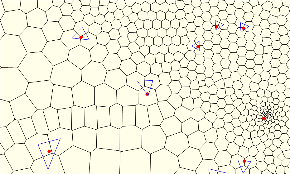
The following programs assist in setup and use of the MODFLOW postprocessors that are listed above. Some of them calculate secondary observations (particularly temporal and spatial differences) that are used in formulating a multiple component objective function. Note, in particular, programs that calculate spatial interpolation factors from a quadtree-refined or arbitrary DISV grid to the sites at which field measurements were made.
Barycentric interpolation (undertaken by MF6INTFAC) from the centres of an ALGOMESH grid to the sites of observation wells. |
The following tables contain members of the groundwater utility suite that are useful in their own right. Structured grid
MODFLOW-USG
MODFLOW 6
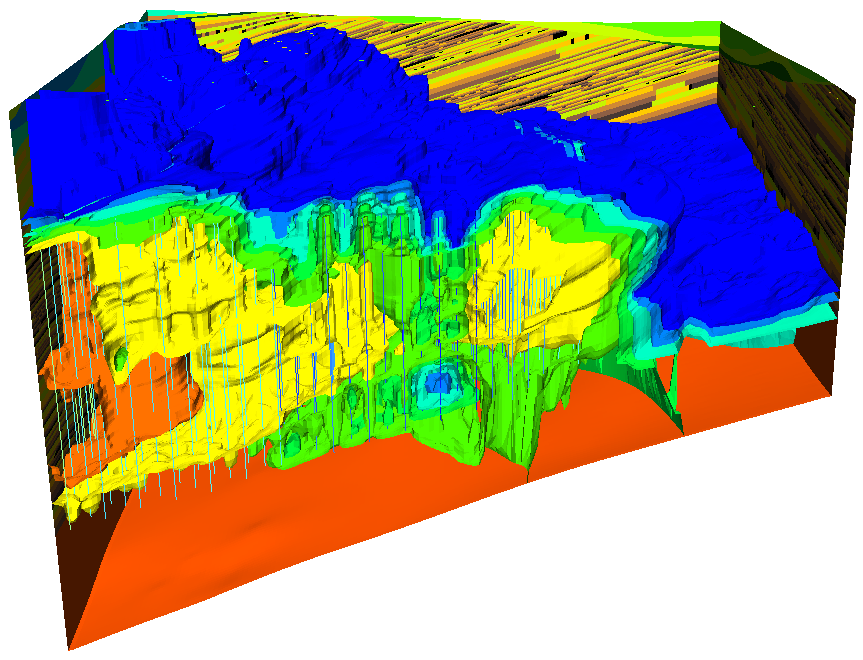
3D contours of heads calculated by MODFLOW-USG displayed in PARAVIEW. |