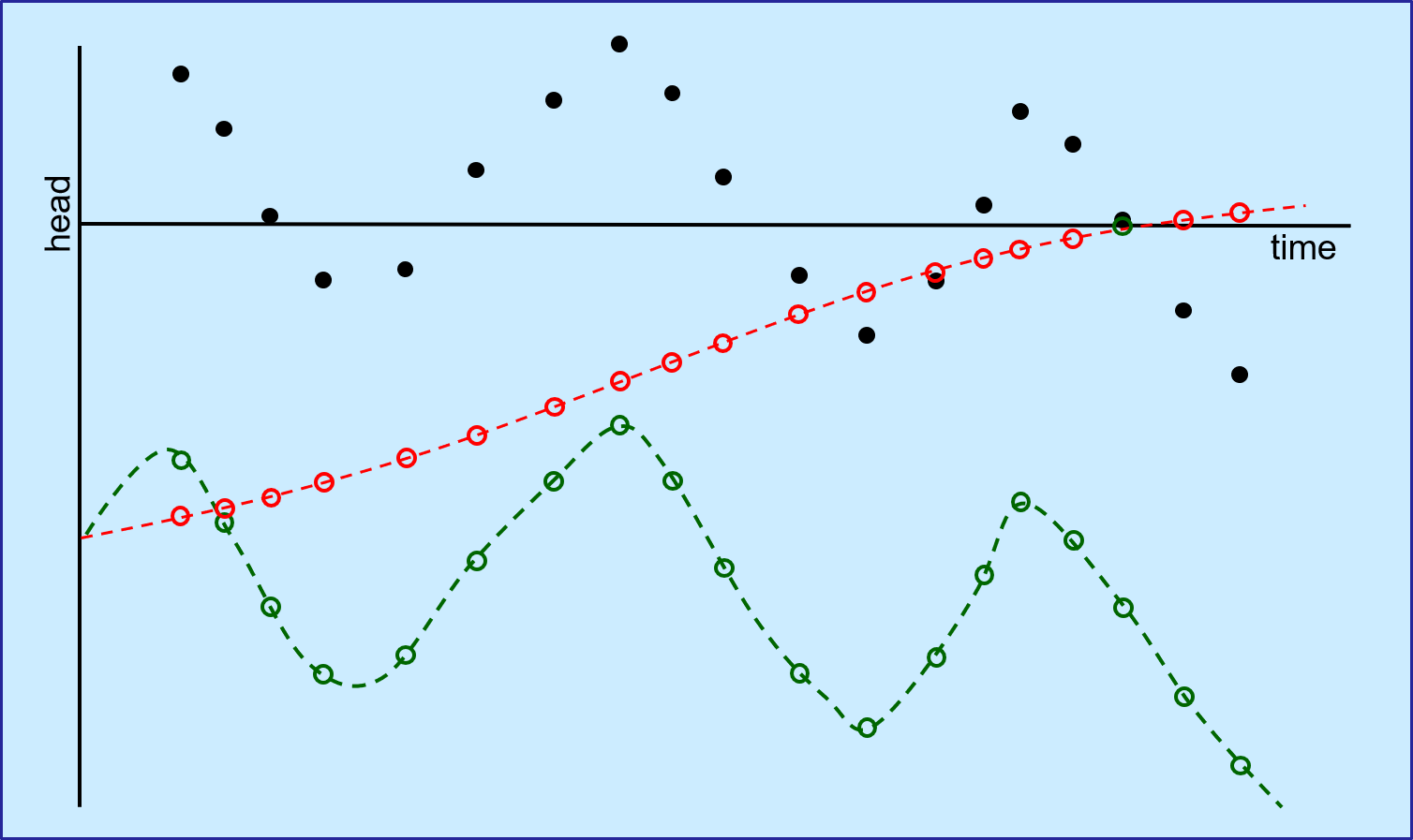
Suppose that you are calibrating a transient groundwater model. Suppose further that it is important for the model to calculate seasonal variations in groundwater levels with as much integrity as available information allows. It is important, therefore, that PEST encourage the model to replicate past seasonal groundwater variations. Furthermore, the model must be capable of replicating these variations, even if it cannot fit actual heads exactly because of model imperfections which may compromise this.

Under these circumstances, which of the following comprises the better fit between model outputs and historical measurements of system head (shown as black dots)?

Measured (black) and model-calculated heads using two different objective function formulations.

In both cases, model-calculated heads start from the same value. This may be a value that is inherited from a previous inversion, or achieved through simultaneous transient and steady-state calibration. However some model imperfection (perhaps a failure to represent local hydraulic conductivity heterogeneity, or an erroneous nearby boundary condition) may make it difficult for the model to replicate local average groundwater levels.

The red curve shows the results of calibrating against heads. That is, groundwater-calculated heads are matched to observed heads. By insisting that measured heads be replicated by the model over the calibration time period, perhaps PEST can slowly drag model-calculated heads to the correct level over the simulation time so that model-to-measurement head residuals are minimised (though hardly reduced to a very low value). This may require introduction of a high value of specific yield, and adjustment of recharge model parameters to values that mitigate seasonal recharge variations. This is not good.

Alternatively, suppose that PEST is explicitly asked to match measured and model-calculated head differences - either differences between sequential heads or differences between each head and the first measured head. In this case, PEST will probably estimate reasonable values of specific yield and recharge parameters because of the direct link between these parameters and temporal changes in model heads. When using the model to make management-salient predictions, perhaps the average head value can be overlooked or corrected. However there can be some confidence that the model's ability to replicate seasonal head variations isn't too bad.

To achieve the green curve as an outcome of history-matching, measured heads must be processed before they are introduced to a PEST control file. Model-calculated heads must be similarly processed by a model postprocessor on each occasion that the model is run. The temporal head differences that are obtained in this way must be placed into their own observation group and weighed for visibility in the total objective function (which may or may not include directly-measured and corresponding calculated heads as well).

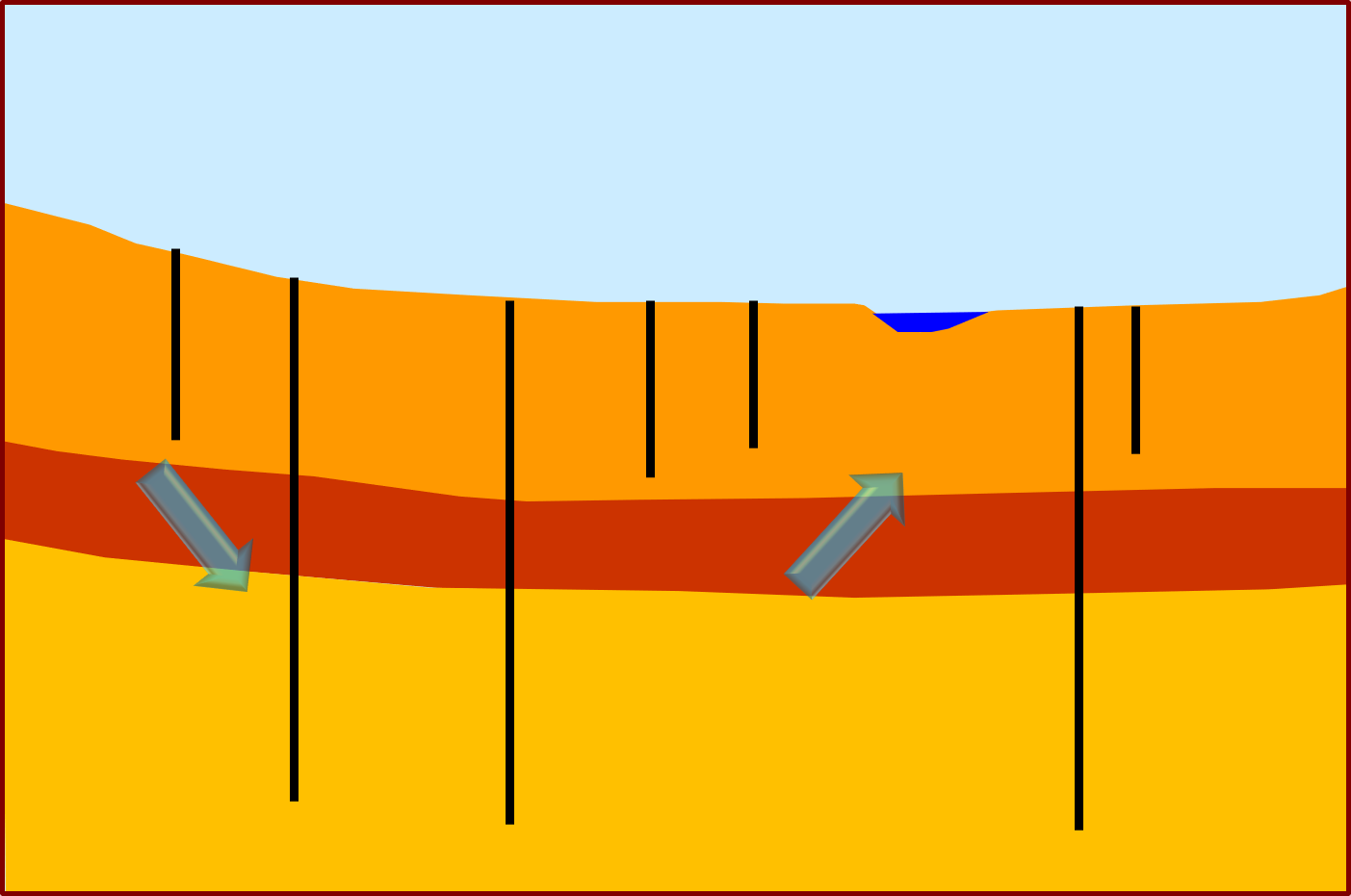
In the picture below, an upper and lower aquifer are tapped by a number of boreholes. These aquifers are separated by an aquitard. In some groundwater management contexts, the vertical hydraulic conductivity of an aquitard such as this may be the hydraulic property of greatest management interest. The aquitard may (or may not) protect the river from excess pumping in the lower aquifer. And/or it may diminish the effects of agricultural contamination of the upper aquifer on the quality of water that is extracted from the lower aquifer.

An aquitard separating two aquifers.

In most modelling contexts, vertical hydraulic conductivities of aquitards are very difficult to estimate.

We have said elsewhere that environmental simulation should be focussed on inquiry. So a modeller should ask him/herself from where, in the history-matching dataset, can information on the vertical hydraulic conductivity of the aquitard be harvested?

This information can be harvested from subtle differences in head between the upper and lower aquifers. Perhaps these differences are not directly measured; they may have to be calculated from head measurements in individual wells (perhaps averaged over time). Regardless of how they are obtained, these head differences should be placed into their own observation group and weighted for visibility in the overall objective function. Furthermore, these weights may need to be high if head differences are small. PEST is therefore given the opportunity to replicate these differences, even if it has difficulty in replicating heads in individual wells because of local model structural or parameterisation imperfections. By replicating these vertical head differences, estimates of aquitard vertical hydraulic conductivity are likely to have as much integrity as the limited calibration dataset allows.

Ask yourself:

•What does this model need to predict?

•What data is most informative of this prediction?

•How can the inverse problem be formulated in a way that harvests this information?

This can get subtle.

Suppose that environmental management will rely heavily on one or a number of statistical indicators of water body health. Flow or water level duration statistics are often used for this purpose. If such a statistic is to be used for future system management, then it is incumbent on a modeller to match historical "observations" of this same statistic during the history-matching process. The model is thus "tuned" to the decision-support role that it must provide. Alternatively, if structural defects impede calculation of this static, this becomes apparent during the history-matching process.

A good rule of thumb is "include in the calibration process that which the model is required to predict".

Another rule of thumb pertains to how observations are subdivided into observation groups.

Observations of different types often contain information that pertains to different parameters. Hence they should be placed into different groups which are then weighted for visibility in the total objective function. The same applies to observations at different locations. For example, heads in an upper aquifer may inform different parameters from heads in a lower aquifer. They should therefore be placed into different groups, and each of these groups weighted for visibility. Inter-layer head differences (if available and if useful) should also be placed into their own observation group and weighted for visibility in the total objective function.

The PWTADJ1 utility that is supplied with the PEST suite can be used to balance observation group weighting so that all observation groups have the same objective function visibility at the commencement of the history-matching process.

It was stated elsewhere that the weight assigned to a measurement should be inversely proportional to the standard deviation of noise associated with that measurement, and that the same constant of proportionality should prevail for all measurements. Theoretically, this weights assignment strategy minimises predictive error variance.

Recommendations and rules of thumb that are provided above seem to violate this theory.

The PEST book, and publications cited therein, points out that this is not necessarily the case. It would be the case if simulators could replicate environmental behaviour exactly. However they cannot do this. Model outputs come with so-called "structural noise". This noise displays a high, but unknown, degree of spatial and temporal correlation. If we knew the covariance matrix of structural noise, then we could use this covariance matrix in place of measurement weights when subjecting a model to history-matching. Unfortunately, it is unknown to us.

What we do know, however, is that some functions of model outputs are more immune to model structural imperfections than others. In general, models are better at calculating spatial and temporal differences than they are at calculating absolutes. It follows that these differences deserve visibility in the objective function. Perhaps they should also be the drivers of model-based environmental management.

Similarly, as discussed above, if model-based management relies on a model's ability to compute certain indicative statistics, then measurements of past system behaviour should be purposefully mined for information that pertains to these statistics. This is done through well-designed history-matching.

It is an inconvenient but important truth that no model can calculate everything equally well. A modeller may therefore need to choose which of its predictions should be most immune from predictive bias. Tuning a model to the predictions that are required of it makes a lot of sense.

Of course, these considerations do not remove the imperative to give smaller weights to measurements that are less trustworthy. In general, the requirement that weights be inversely proportional to the standard deviations of measurement noise should apply within a particular observation group, but is less applicable between observation groups.