Tikhonov regularisation seeks uniqueness in the opposite way to singular value decomposition (SVD). Whereas SVD decreases the dimensionality of estimable parameter space, Tikhonov regularisation increases the number of "measurements" through which parameters are estimated. It supplements the calibration dataset with at least one new measurement for every parameter (often more than this). These "measurements" are actually the encapsulation of a modeller's prior knowledge about parameters, and are therefore an expression of the prior parameter probability distribution. To be sure, this knowledge is often vague. However, when working with many parameters, a modeller cannot escape the responsibility of assigning a prior probability distribution to parameters, even if this distribution assigns wide uncertainties to individual parameters. A modeller's hydrogeological knowledge is like a torch that illuminates the dark null space. It may not show much, but it does show something. In fact it shows all that can be known about the occupants of this space.

One of the most attractive features of Tikhonov regularisation is that its path to parameter and predictive uniqueness is flexible. It allows expert knowledge to be expressed in creative ways that reflect the hydrogeological nuances of a particular site. This is one of the things that make Tikhonov regularisation a more attractive regularisation option than SVD.

Moreover, when implemented in a certain way, it can be shown that Tikhonov regularisation is mathematically equivalent to SVD conducted on Karhunen-Loѐve-transformed model parameters. This implementation of Tikhonov regularisation is sometimes referred to as "Bayesian Tikhonov".

Tikhonov regularisation adds two important ingredients to the highly-parameterised inversion process.

Firstly, it provides a fall-back position for all parameters. This fall-back position can be comprised of an individual value for each parameter. Or it can be comprised of relationships between parameters (often of spatial uniformity) that should prevail unless the calibration dataset provides evidence to the contrary.

The second thing that Tikhonov regularisation brings to the inversion process is guidance on how departures from this preferred condition can occur, should this be required for model outputs to fit field measurements. Ideally, departures should occur in ways that make hydrogeological sense, and that are therefore in accordance with the prior parameter probability distribution.

Addition of these two important ingredients to the calibration soup may sound difficult. However it is easy to do. It can be done by simply enhancing the inversion process with a set of appropriately weighted "observations" that pertain directly to parameters. Misfitting of these observations contributes to model-to-measurement misfit, and is therefore penalised.

Tikhonov regularisation can be linear or nonlinear. In the former case it can be introduced to a PEST input dataset as prior information (i.e. linear PEST-calculated functions of parameters for which a modeller provides "observed" values). In the latter case, the model must itself calculate appropriate functions of parameters which are then matched to modeller-supplied "observed" values of these functions.

When using the PEST suite, the easiest form of Tikhonov regularisation to apply is Bayesian Tikhonov. A preferred value is ascribed to each parameter. This is its prior mean value (i.e. its "expected value" from the point of view of its prior probability distribution). Meanwhile, a covariance matrix is used instead of weights for these observations. This covariance matrix is the one that features in the prior parameter probability distribution (assuming that this probability distribution is Gaussian). See the PEST book, or videos on the mathematics of PEST, for further details.

As stated above, the beauty of Tikhonov regularisation lies in its flexibility and (if necessary) its sophistication. This is highly developed in fields such as image processing where it forms the basis for algorithms such as sharpness filtering.

In the groundwater context, Tikhonov constraints may be employed to suppress the emergence of heterogeneity in one place rather than in another. However, it is in the nature of Tikhonov regularisation that this "advice" to the inversion process can be ignored if it compromises the ability of model outputs to fit field measurements of system state or flux.

Tikhonov constraints can also induce the inversion process to align the direction of emergent heterogeneity with that of known structural features. At the same time, it may be used to suggest to the inversion process that permeable features should have sharp boundaries in certain parts of the model domain, but be more diffuse at other locations. Considerable effort has been devoted to the derivation of nonlinear parameter functions which are able to express these conditions - especially in the field of geophysical data interpretation where Tikhonov regularisation has been used since its inception.

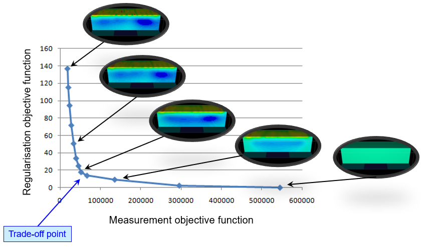
An attractive feature of Tikhonov regularisation as implemented in PEST is the ease with which over-fitting can be prevented. Before describing this, we briefly introduce the concept of "objective function".

An objective function measures model-to-measurement misfit. In its simplest formulation it is the sum of squared weighted residuals (i.e. differences) between model outputs and field measurements. The lower is the objective function, the better are model outputs matched to their field-measured counterparts.

When PEST is undertaking Tikhonov regularisation, it employs two objective functions. That which specifies model-to-measurement misfit is referred to as the "measurement objective function". That which specifies departures of parameters from their preferred values is referred to as the "regularisation objective function".

Over-fitting occurs if the measurement objective function is too low. The problem with over-fitting is that this fit comes at the cost of parameter value credibility. The regularisation objective function therefore rises. Attainment of the "best" fit between model outputs and field measurements therefore requires that the measurement and regularisation objective functions be traded off against each other. If one is plotted against the other, this trade-off can be done manually. Geophysicists sometimes refer to this trade-off curve as the "L" curve. The optimal location along this curve is often considered to be where it starts to rise steeply. It is at this point that the cost of attaining a better fit between model outputs and field measurements is rapidly increasing stupidity of parameter values. PEST allows you to plot this curve when run in "Pareto" mode.

The L curve applied to interpretation of 3D resistivity data.

In most case of groundwater model calibration, production of an L curve is inefficient. So PEST offers a simpler alternative. This alternative is invoked when PEST is run in "regularisation" mode. The modeller nominates a measurement objective function that reflects the amount of noise that accompanies field measurements. PEST then seeks to attain this objective function, but will not allow estimation of parameters that reduce the measurement objective function below this value. Meanwhile, PEST finds the smallest regularisation objective function that is compatible with this user-nominated "target measurement objective function".

In implementing this process, a modeller has the ability to plot an approximate "L" curve by monitoring measurement and regularisation objective functions attained during each iteration of the inversion process. If the final target measurement objective function turns out to be too low (because parameters must adopt unrealistic values to achieve it), then parameter values from previous iterations that correspond to higher measurement objective functions can be selected instead.