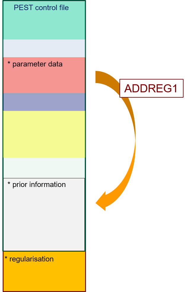
Once you have added pilot point parameters to a PEST input dataset (and checked your work with PESTCHEK), you must add Tikhonov regularisation to the PEST control file. The easiest way to do this is to use the ADDREG1 or ADDREG2 utility. These add a prior information equation for every pilot point parameter. Through this equation, the respective pilot point parameter is endowed with a preferred value that is equal to its initial value. As a consequence, every parameter will adhere to its initial value during the inversion process unless the measurement dataset says otherwise.

A modeller therefore needs to ensure that initial parameter values are prior mean parameter values. This does not make these values right. It simply minimises their potential for wrongness from an expert knowledge point of view. (This potential may be large; it depends on the prior uncertainty of each parameter.)

Always ensure that the PEST control file has a "singular value decomposition" or LSQR section. If using singular value decomposition, ensure that the EIGTHRESH variable in the "singular value decomposition" section is set to 5E-7 or greater. This protects the regularised inversion process from numerical instability.

When ADDREG1 or ADDREG2 add prior information to a PEST control file, they assign a default weight of 1.0 to each equation. There is a message for PEST in this. The message is that each one of these equations should be enforced independently of the other equations. This independence applies whether equations pertain to pilot points which are close together or far apart.

However, this is not the way that the subsurface operates. Generally, points that are close together possess hydraulic properties that are similar. This notion is encapsulated in a variogram. If the information content of field data requires that heterogeneity emerge in a certain part of the model domain, then ideally this variogram should be respected as it emerges. That is, heterogeneity should show spatial correlation as it arises, rather than arising on a point-by-point basis.

For spatial correlation to prevail as heterogeneity arises, each prior information group that cites pilot point parameters should be awarded a covariance matrix. This replaces weights in calculation of the regularisation component of the objective function.

We explain how to build a covariance matrix below. Once built, the covariance matrix is stored in a file. The name of this file should be placed opposite the name of the pertinent observation group (i.e. prior information group) in the "observation groups" section of the PEST control file. PEST then knows to use this covariance matrix in calculating the contribution to the objective function made by that prior information group rather than weights ascribed to individual equations.

The "observation groups" section of a PEST control file is shown below. In this example, covariance matrices are assigned to three observation groups that are used for regularisation purposes. Notice how the same matrix can be employed by more than one group. This can happen only when each group has the same number of equations, and the parameters that are cited in the equations that belong to each group are hosted by the same set of pilot points.

The PEST groundwater utility suite provides four programs that build covariance matrices for families of pilot points. Two other programs can provide further assistance. All of these programs are listed in the following table.

Using PPCOV and PPCOV3D is easy. You need to prepare a "pilot points file" that lists the names and coordinates of pilot points. (You will already have built one of these files if you use PLPROC as a simulator preprocessor.) You will also need a "structure file". The following figure shows such a file. It is easy to build this file using a text editor. See Part B of the manual of the groundwater utilities for further details.

Use of PPCOV_SVA and PPCOV3D_SVA is not much harder. ("SVA" stands for "spatially varying anisotropy".) These utilities require a "pilot point statistical specification file". This provides variogram parameters at the location of every pilot point. The MKPPSTAT utility can make this file for you; modify the file that it produces as you see fit. Here is part of a pilot points statistical specification file for a set of 2D pilot points.

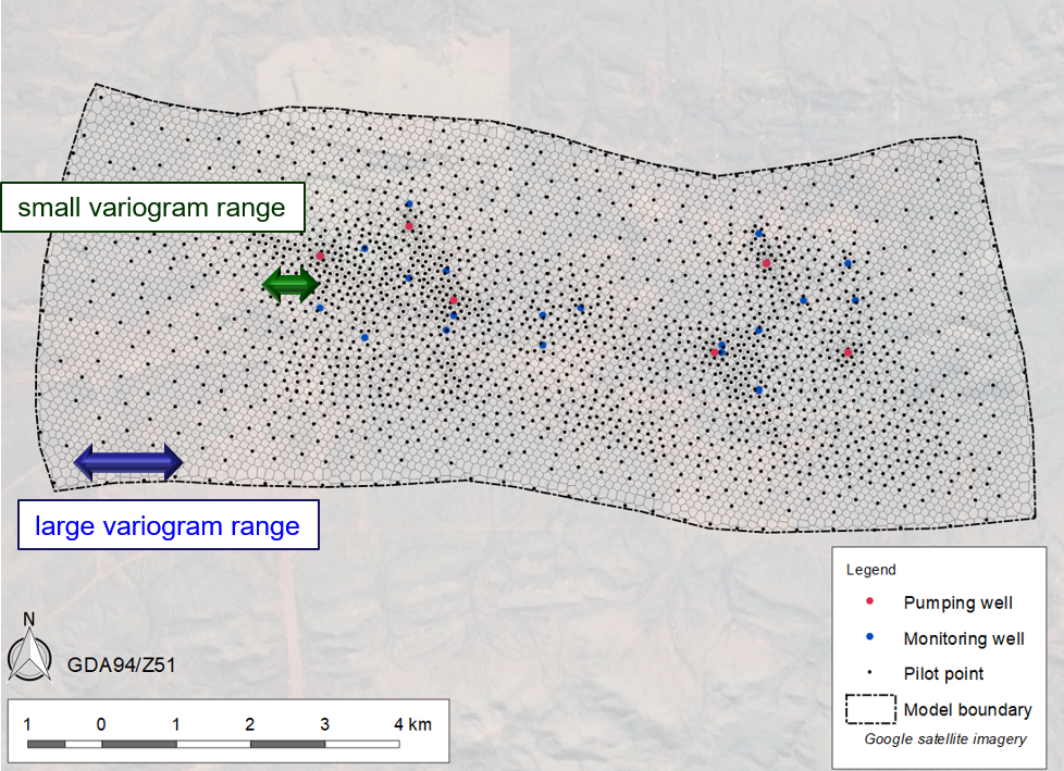
Why would you want variogram properties to vary in space? Here are a couple of good reasons.

Pilot point density

When distributing pilot points throughout a model domain, it is often a good idea to have a higher spatial density of pilot points where the spatial density of information is larger. Pilot point parameters can therefore provide receptacles for the increased density of information. Hence it makes sense to increase pilot point spatial density where the density of observation wells is higher.

Now let's look at what is implied by this pilot point emplacement philosophy. Implied in a higher pilot point spatial density is the assumption that heterogeneity may emerge at the same scale. This is not to say that you expect the subsurface to be any less heterogeneous in those parts of the model domain where pilot point densities are lower because of lower information density. It's just that there is insufficient information to support the emergence of finer scale heterogeneity at these locations. Furthermore, if these parts of the model domain are far away from locations at which model predictions are required, then nothing is lost by representing only broad scale heterogeneity using broadly spaced pilot points and a local variogram range to match.

It makes sense, therefore, for the spatial covariance between pilot point parameters to reflect the local separation of pilot points. A covariance matrix can be built to put this into effect. Meanwhile, the MKPPSTAT utility can calculate local variogram ranges that reflect local pilot point densities.

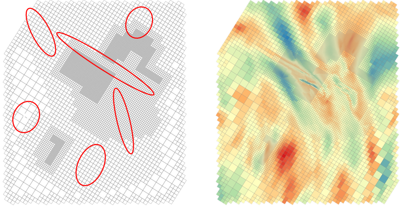
Anisotropy

There are geological contexts where it makes sense for the shape of emergent and/or random heterogeneity to be more elongate in one direction than in the orthogonal direction. River channels are one of these contexts. Areas that may be intersected by geological structures are another of these contexts.

Using PPCOV_SVA and PPCOV3D_SVA you can build a covariance matrix that reflects this. Patterns of heterogeneity that emerge through calibration, or that are used to represent hydrogeological uncertainty, can then express this. In some areas the principle axis of anisotropy may be oriented in one direction, while it may be oriented in another direction in other areas.

In the early days of PEST's support for pilot points, utilities were provided for automatic addition of "preferred difference" regularisation to a PEST control file. Using this regularisation protocol, a number of prior information equations are introduced to the PEST control file for each pilot point parameter. Each of these equations subtracts the value of a pilot point parameter from the value of a neighbouring pilot point parameter. The difference is equated to zero. The larger is the separation between pilot points, the lower is the weight that is assigned to the prior information equation.

An advantage of this mode of regularisation is that a modeller can avoid assigning a preferred value to each pilot point. This seems appropriate if he/she is unsure of what this preferred value should be. Instead, he/she may feel much more comfortable in suggesting to the inversion process (through regularisation) that parameter homogeneity should prevail unless there is information to the contrary in the calibration dataset.

A disadvantage of preferred difference regularisation is the number of prior information equations that are required to implement it. Suppose that a preferred difference of zero is requested between each pilot point and its five nearest neighbours. Then the number of prior information equations that implement preferred difference regularisation is five times the number of pilot point parameters. This increases the memory that is required to store the Jacobian matrix.

It is possible to have the best of both worlds if pilot points are parameterised as multipliers. Parameterise (and estimate) the value of the hydraulic property that is assigned to a whole layer or zone. Then use pilot point multipliers to add heterogeneity to this layer or zone. (This is easily done using PLPROC.) You can use preferred value regularisation together with a covariance matrix for the pilot point parameters. The preferred value is 1.0.