Conceptually, achievement of inverse problem uniqueness requires a reduction in the number of parameters that must be estimated, or an increase in the number of measurements on which their estimation is based. Basic mathematics shows that the number of measurements must exceed the number of estimable parameters for achievement of parameter uniqueness. In most cases, measurements should exceed parameters by a considerable margin for parameter uniqueness to be attained.

As we have discussed, parameter simplification can be achieved manually through manual regularisation. However there are smarter ways to achieve parameter simplification.

Manual regularisation recognises that the information content of a calibration dataset generally supports estimation of combinations of parameters. At the same time, there are other combinations of parameters which are beyond the reach of the inversion process. The combinations which are estimable are normally broadscale parameter averages, or local spatial averages near locations at which data have been gathered. A parsimonious zonation scheme may be designed to capture these averages. The combinations that are inestimable often pertain to local hydraulic property detail (for example local differences between neighbouring parameters), especially at locations that are removed from the sites at which measurements were made.

This notion is mathematically formalised through singular value decomposition.

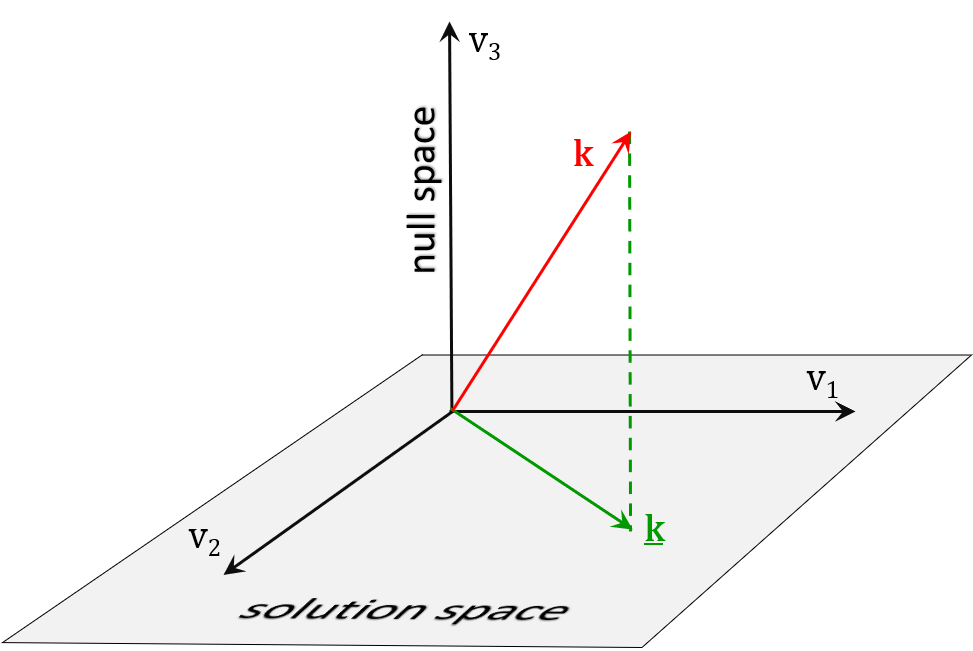
Singular value decomposition (or SVD for short) is a complex numerical operation that is performed on a matrix. When calibrating a groundwater model it is performed on the Jacobian matrix - also known as the sensitivity matrix. This matrix contains the sensitivity of every observation-pertinent model output ("observations" for short) to every model parameter. The larger the number of parameters, and the larger the number of observations that comprise a calibration dataset, the larger is this matrix.

SVD partitions parameter space into two orthogonal subspaces. The first subspace is comprised of combinations of parameters that are uniquely estimable on the basis of the calibration dataset. This space is referred to as "the solution space". The second is comprised of combinations of parameters that are uninformed by the calibration dataset. This space is referred to as "the null space". The dimensionalities of these two spaces add up to the number of parameters. In most modelling contexts, the dimensionality of the solution space is much less than that of the null space. When calibrating a model, only combinations of parameters that occupy the solution space are adjusted. Those that occupy the null space are left alone.

This neat subdivision of parameter space into two orthogonal subspaces has profound consequences.

Firstly, parameter simplification is automated. A modeller does not need to guess in advance of the parameterisation process what can be estimated and what cannot be estimated. When parameterising a model, a modeller can include whatever hydraulic property detail that he/she considers necessary. This can include detail that may or may not be estimable. For reasons already stated, it should include detail to which predictions of management interest are sensitive, regardless of the estimability (or otherwise) of this detail.

SVD separates what can be estimated from what cannot be estimated. What can be estimated is not generally describable as individual parameters, but as combinations of parameters. These are vectors that span the solution space; combinations of parameters are the elements of these vectors. The inversion process estimates factors by which these combinations are multiplied, and then combines them.

Secondly, parameter simplification achieved in this way can be shown to be optimal. Predictions made with a model that is calibrated using SVD are indeed of minimised error variance. (More on this below.)

Thirdly, SVD explains the relationship between unknown "real-world" parameters, and parameters that are estimable from a calibration dataset. In particular, it shows that we cannot know the hydraulic properties of "reality". All that we can know is the projection of these properties onto a smaller dimensional subspace, this being the solution space.

Parameters estimated by SVD are the projection of real-world parameters onto the solution space.

However one of the nicest things about SVD is its numerical elegance. Solution of an ill-posed inverse problem requires inversion of a large matrix. In partitioning the Jacobian matrix, SVD alters the matrix that it must invert to ensure that it is invertible. The inversion process is therefore numerically stable, regardless of how ill-posed is an inverse problem.

There are other nice things about SVD as well. Not only does it isolate a uniquely estimable set of parameter combinations, and then estimate values for these combinations (from which values of actual parameters can be calculated). It identifies combinations of observations that inform combinations of parameters. Flow of information from measurements to parameters can therefore be tracked. Theory associated with its deployment, can also indicate where overfitting starts to occur and why over-fitting is a problem.

"The number of estimable combinations of parameters" is another gift from SVD. This is the number of useable items of information in a calibration dataset. This is often handy to know.

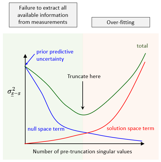
Unfortunately, use of SVD to calibrate a model is accompanied by some difficulties.

The first of these difficulties is statistical characterisation of parameters.

We have already said that use of a large number of parameters is not a problem for SVD. However, these parameters must be assigned a prior probability distribution. This is something that cannot be escaped whether doing model calibration or uncertainty analysis. History-matching cannot provide unique values for all parameters - especially those which represent small-scale, but nevertheless important, potential hydraulic property heterogeneity. Combinations of parameters that are not informed by a calibration dataset (and therefore occupy the null space), can only be informed by us. This information is necessarily probabilistic. It is encapsulated in the prior parameter probability distribution.

Unfortunately, when calibrating a model using SVD, the promise of minimised predictive error variance can only be delivered if native model parameters are transformed into a secondary set of parameters. It is this secondary set of parameters which is estimated using SVD. Calibrated native model parameters are then back-calculated from these.

The transformation through which secondary parameters are calculated from primary parameters is known as the Karhunen-Loѐve transformation. It requires eigencomponent decomposition of the covariance matrix that characterises the prior parameter probability distribution. This is not easy to undertake where parameter numbers are very large. It also requires that certain assumptions be made about the prior parameter probability distribution - assumptions that are a little inflexible in light of the complex patterns of heterogeneity that characterise real world systems.

The second problem is prevention of over-fitting. The theory behind SVD-based regularisation shows with great mathematical elegance what over-fitting is, and what damage it can do to the parameter estimation process. If the solution space is declared to be too large, then measurement noise can be amplified when estimating parameters. Amplified measurement noise can hide the information content of measurements. Prevention of this occurrence depends on selection of an appropriate "singular value truncation level". This determines the dimensionality of the solution space, and hence the number of pieces of information that are admitted into the inversion process. In practice, selection of the optimum singular value truncation level is easier said than done. Furthermore, it is a rather inconvenient way to prevent over-fitting.

SVD-based analysis of over-fitting. See the PEST book for details.

SVD (or methods that are closely related to it) are at the heart of all modern-day inversion and uncertainty analysis algorithms which require manipulation of many parameters for their conceptual integrity. It is SVD that assures the numerical integrity of these algorithms. So while SVD may not be selected as the primary regularisation device when conducting regularised inversion (some form of Tikhonov regularisation is normally employed), it comprises the numerical engine of any inversion process that guarantees success of Tikhonov regularisation.

Inversion and uncertainty analysis require the inversion of large matrices. Where an inverse problem is ill-posed, or verges on being ill-posed, matrix inversion becomes unstable at best and impossible at worst. However by basing the matrix inversion process on SVD, an approximate matrix inverse can always be derived which is often superior to the real inverse. (SVD ensures that numerical noise is not amplified when inverting a singular or near-singular matrix.) What is more, modern-day implementations of SVD (which use clever algorithms such as randomised SVD) can be numerically very fast indeed.