"GENLINPRED" stands for "general linear analysis".

GENLINPRED automates performance of a number of types of linear analysis, including the following:

•parameter and predictive uncertainty;

•relative parameter uncertainty variance reduction;

•relative parameter error variance reduction;

•parameter identifiability;

•parameter contributions to predictive uncertainty;

•parameter contributions to predictive error variance.

In performing these analyses, GENLINPRED runs many of the linear analysis utilities that are discussed on previous pages. Its analyses are useful and easy to perform. However more targeted analyses can be performed if a user runs these utilities him/herself.

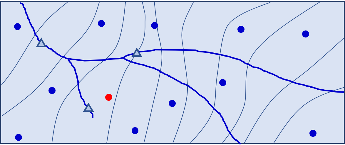
Suppose that you have tried to calibrate a model, but you are frustrated because there are one or two observations in critical places that you are unable to fit well. These observations may resemble, in type and location, predictions that are important for the decision-support role that the model is intended to play.

For example, suppose that you cannot fit heads in the red observation well in the figure below. Does this indicate a competition with other head and/or flow observations, so that parameters cannot accept values that allow a good fit with all of them at the same time? If this is the case, then which observations are providing this competition? Or is failure to fit the red observation an outcome of local model defects?

The OBSCOMP utility that is supplied with PEST uses sensitivities that are recorded in a Jacobian matrix file to help answer this question. As for so many other utilities, the focus is on flow of information. However OBSCOMP addresses the question "why isn't the information flowing?" The answer may be erroneous data. Or it may be an erroneous model. The answer cannot be definitive, but OBSCOMP can show you where to look.

PEST records composite parameter sensitivities in a file named case.sen, where case is the filename base of the PEST control file. (This is normally called a "SEN file".) In the early days of PEST, before numerical regularisation was used to attain parameter uniqueness, the contents of a SEN file could be used to identify parameters which should be removed from the inversion process. A good rule of thumb was that if the ratio of a parameter's composite sensitivity to that of the parameter of greatest composite sensitivity was less than about 1 in 100, then the parameter is probably not uniquely estimable. It should therefore be fixed or tied to another parameter.

Despite the ubiquitous use of numerical regularisation these days, composite parameter sensitivities can still be useful for problem diagnosis.

If a parameter has a very high composite sensitivity, this may indicate corrupted calculation of finite-difference derivatives with respect to that parameter. Its super-sensitivity will be apparent from the SEN file. Alternatively, its super-sensitivity may be an outcome of the way in which the inverse problem is formulated, or the fact that the parameter's units are such that its value is very small. Super-sensitivity of one parameter can make it difficult for PEST to estimate values for other parameters. So perhaps the offending parameter should be log-transformed in the PEST control file. Or perhaps it should be given a larger value in the PEST control file, and then scaled down for the model using the SCALE variable that is ascribed to that parameter in the "parameter data" section of the PEST control file.

Very small composite parameter sensitivities may also indicate the need for some degree of inverse problem reformulation. However, these may be difficult to see if the inverse problem includes Tikhonov regularisation. (The whole idea of Tikhonov regularisation is to ensure that no parameter is very insensitive.) Artificial parameter insensitivity can be discovered if you remove regularisation from a PEST control file using the SUBREG1 utility, and then re-compute composite parameter sensitivities. (Run PEST with NOPTMAX set to -1, and use the "/i" switch on the PEST command line to extract sensitivities from an existing Jacobian matrix file to make this process very quick.) If you think that a parameter should be more sensitive than it presently is, then log transform it (if it is not already log transformed). Alternatively, if it cannot be log transformed because it may become negative, use the SCALE variable in the opposite way to that discussed above.

Some useful matrices

If PEST is run in "estimation" mode, and if no form of regularisation is used, then it records three matrices at the end of its run record file. These are:

•the posterior parameter covariance matrix;

•the posterior parameter correlation coefficient matrix;

•eigenvectors and eigenvalues of the parameter covariance matrix.

Prior parameter uncertainties are not used to compute these matrices as the inverse problem is presumed to be well-posed. If it turns out that the inverse problem is not well-posed, then these matrices cannot be computed. PEST will inform you of this. (Then use PREDUNC7 to compute posterior parameter uncertainties instead.)

If an inverse problem is nearly ill-posed, then the contents of these matrices can diagnose this condition. At the same time, they can indicate which parameters are causing problems. These tend to be parameters that exhibit high posterior correlation with other parameters, or that feature in posterior covariance matrix eigenvectors for which corresponding eigenvalues are large. See PEST documentation for more details.

The EIGPROC utility

EIGPROC is supplied with PEST. It collects information on parameter sensitivities, and on eigencomponents of the posterior parameter covariance matrix. It summarises this information in a way that allows a modeller to understand the extent to which a parameter's value is informed (or is not informed) by the current calibration dataset.

INFSTAT and INFSTAT1

INFSTAT uses the contents of a Jacobian matrix to calculate observation influence statistics that include:

•Cook's D;

•DFBETAS;

•Hadi's statistic.

These provide a measure of the importance of different observations that comprise a calibration dataset. See Part 2 of the PEST manual for more details if you are interested. Use of INFSTAT assumes that an inverse problem is well-posed. INFSTAT1 extends the analysis to ill-posed inverse problems.