In general, predictive error is of less interest to us than predictive uncertainty. However its analysis can sometimes be interesting.

"Error" describes how much a prediction made by a calibrated model may be wrong. If calibration is implemented properly, the magnitude of potential predictive error is similar to the magnitude of posterior predictive uncertainty. (See the PEST book for more details.)

Consider a prediction s whose sensitivities to model parameters k are stored in the vector y. The error variance of s is denoted by the symbol σ2s-s where s refers to the prediction made by the calibrated model and s refers to the true (but unknown) value of the prediction. It can be shown that:

σ2s-s = σ2kyTV2VT2y + σ2εyTV1S-21VT1y

In the above equation, σ2k characterises the prior uncertainty of parameters while σ2ε characterises measurement noise. V1 is an orthogonal matrix whose columns span the solution space of parameter space while V2 is an orthogonal matrix whose columns span the null space of parameter space. These are discovered by subjecting the weighted Jacobian matrix to singular value decomposition. The boundary between these two spaces should be chosen in a way that minimises the error variance of all model predictions.

We use the term "singular value truncation" to identify where subdivision of parameter space into two orthogonal subspaces should occur. Singular values start off large and get smaller. At some point we say "small is equal to zero". This is where the null space is presumed to begin. The null space is spanned by columns of the V2 matrix while the solution space is spanned by columns of the V1 matrix. We refer to the first term on the right of the above equation as the "null space term" and the second term on the right as the "solution space term".

Believe it or not, the above equation is really informative.

Firstly, it explains why over-fitting is bad. Do you see the "-2" superscript in the second term? Small singular values get amplified when they are inverted. If we try to get too much information from data, amplified measurement noise shields that information from view; predictive error variance can then get very large indeed.

Secondly the above equation shows that predictions that are sensitive to solution space parameter components (i.e. the columns of the V1 matrix) have their propensity for predictive error (i.e. their uncertainties) reduced through model calibration. This is not the case for predictions that are sensitive to null space parameter components (i.e. the columns of the V2 matrix). So calibration reduces the uncertainties of some predictions but not that of others. It depends on the prediction.

Thirdly, the relative magnitudes of the above two terms show where the posterior uncertainty of a prediction comes from - the solution space or the null space. That is, whether it comes from contamination of information by measurement noise, or from lack of information.

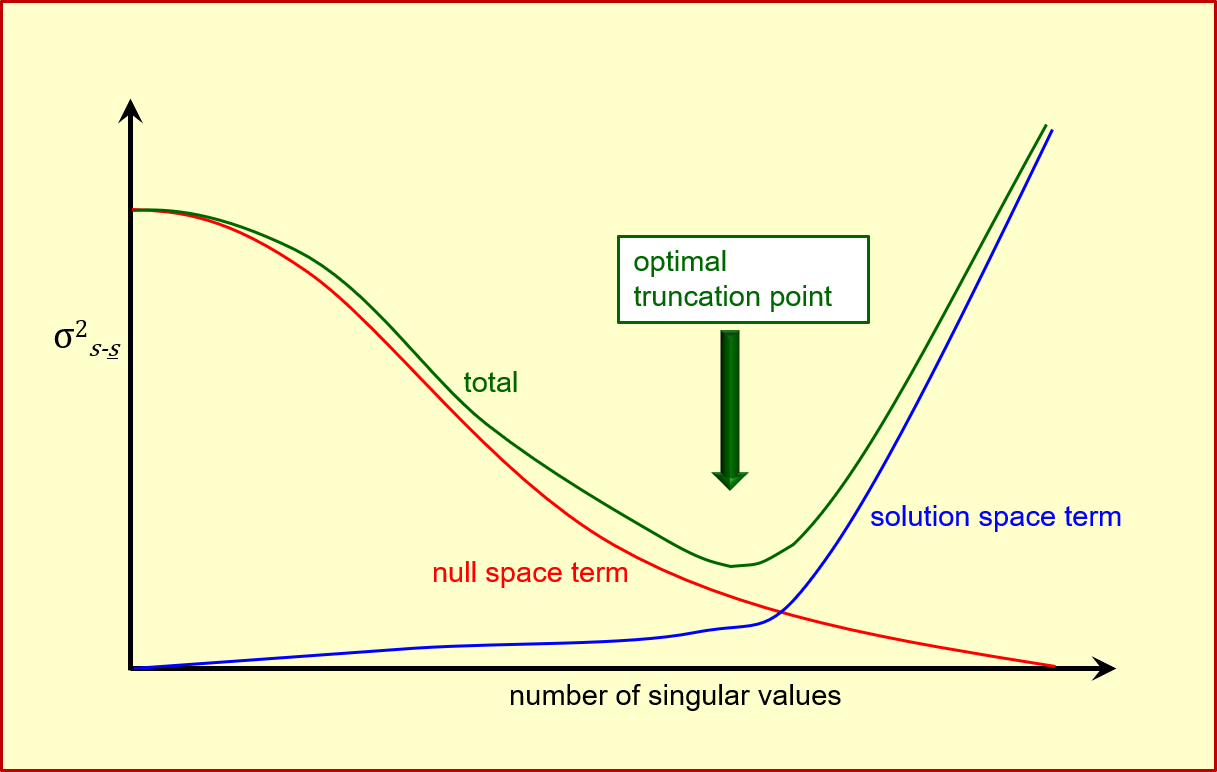
Suppose that we plot the error variance of a prediction of interest against the number of singular values at which partitioning of parameter space into the solution and null space occurs. Points along this curve can be computed by the PREDVAR1 and PREDVAR1A utilities. The curve looks something like this.

Plot of predictive error variance produced by PREDVAR1.

If we underfit a calibration dataset, then our calibrated model lies to the left of the optimal singular value truncation point. If we overfit a calibration dataset, then our calibrated model lies to the right of the optimal singular value truncation point. "Truncation" refers to the singular value index at which the solution space ends and the null space begins. (See the x-axis of the above figure.)

In practice, it is not always easy to know the optimal level of model-to-measurement misfit. This is because we are rarely sure of the level of measurement noise that accompanies a calibration dataset. And we are usually grossly unsure of the level and nature of model-generated structural noise.

Plots such as the above can be informative in other ways. As stated above, at any singular value truncation point (including the optimum truncation point where predictive error variance is approximately equal to the posterior variance of predictive uncertainty) we can see contributions to predictive error variance made by the solution space and null space terms of the predictive error variance equation. In other words we can see whether the uncertainty of a particular prediction is dominated by contamination of information by measurement noise, or by lack of information pertaining to that prediction.

If we do not take model imperfections into account, the number of singular values at which predictive error variance is minimised is the same for all predictions. Hence the ideal number of singular values can be determined without the need to consider any specific prediction. The SUPCALC utility (supplied with PEST) can perform this calculation.

Singular value decomposition allows a modeller to track the flow of information from observations to parameters, and from parameters to model predictions. The theory shows that orthogonal linear combinations of observations are uniquely and entirely informative of orthogonal linear combinations of parameters.  Using PEST jargon, these linear combinations of observations are referred to as "super-observations" while the linear combinations of parameters that they inform are referred to as "super-parameters". Sometimes it is informative to plot the observation components of an individual super-observation in space and time, and the parameter components of an individual super-parameter in space and time.

The following utilities, supplied with PEST, assist in calculation of components of super-observations and super-parameters.

A calibration dataset may contain hundreds, thousands, or even hundreds of thousands of observations. But how many usable pieces of information does it contain?

This question is the same as "what is the optimal dimensionality of the solution space"? Or it can be asked a different way. "How many distinct and orthogonal combinations of parameters are uniquely estimable on the basis of a calibration dataset?"

The SUPCALC utility provides a quick way of answering this question. This can be used as a precursor to SVD-assisted inversion. Or it can be used simply to inquire about the information content of a calibration dataset. It rapidly tries to compute the singular value index at which error variance is minimised.

We define the identifiability of a parameter as the square of the direction cosine between a vector that points along the parameter's axis in parameter space, and the projection of that vector onto the solution space.

Identifiability varies between 0.0 and 1.0. If it is 0.0, then the parameter lies entirely within the null space. The calibration dataset is therefore uninformative of that parameter. If it is 1.0, then the parameter lies entirely within the solution space. The calibration dataset therefore supports unique estimation of that parameter. However this estimate is not without error because the calibration dataset is contaminated by noise.

Parameter identifiabilities often lie between 0.0 and 1.0. This means that the calibration dataset has something to say about a parameter's value, but not enough to estimate it uniquely.

Parameter identifiability can be computed using the IDENTPAR and SSSTAT utilities supplied with PEST. Parameter identifiabilities can be plotted in space, and/or graphed as histograms. These plots can be informative.

However caution must be exercised. Identifiabilities (particularly for some parameters) are sensitive to the number of singular values that separates the solution space from the null space. There is often some doubt as to what this number should be as the minimum of the error variance curve is often shallow and broad.

Another problem is that the identifiability of an individual spatial parameter is not necessarily an indication of flow of information to a particular part of the domain of a model. Suppose that a groundwater model is parameterised using pilot points. The greater the number of points that is used, the less is the identifiability of each individual pilot point parameter.

In many circumstances, a better statistic can be used to monitor flow of information to different parts of a model domain. This is relative parameter uncertainty variance reduction. This, too, is a number between 0.0 and 1.0. However it takes account of the prior probability distribution of model parameters. Where pilot point spatial density is large (because there are lots of pilot points in a particular part of the model domain), then the prior spatial correlation between them is large. Hence discovering something about one pilot point parameter tells us something about neighbouring pilot point parameters. This is taken into account when computing relative parameter uncertainty variance reduction. This statistic is computed by the GENLINPRED utility. (Or you can compute it yourself.)

Nevertheless, there are circumstances, especially where parameterisation is zone-based, where graphs or plots of parameter identifiability can be of considerable didactic worth.

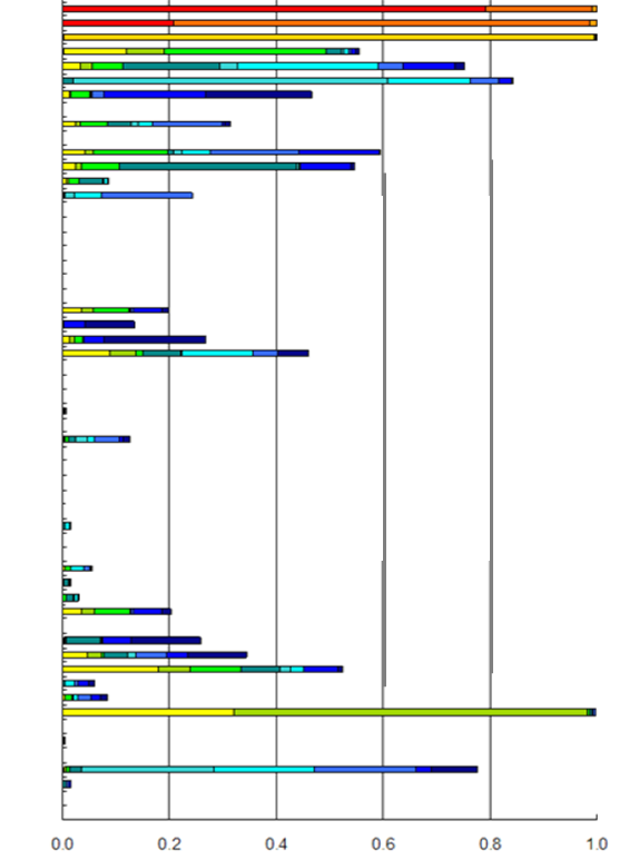
Parameter identifiabilities, colour-coded according to magnitude of projection onto different eigencomponent axes. Warmer colours indicate projection onto axes associated with higher singular values.

(Parameter values are unnamed for confidentiality)

Simulator inadequacies can bias important model predictions in two ways.

The first is through the fact that these defects exist at all.

The second arises from the necessity for model parameters to compensate for these defects as they are adjusted in order for model outputs to fit measured system behaviour. This effect can be rather insidious. A model's defects may not compromise its ability to replicate the past; hence they may remain invisible.

Under certain circumstances, linear analysis can be used to explore this issue. It often reveals the following.

•Some predictions are relatively immune from model defects. For these predictions, if the model can replicate the past, then it can predict the future without bias - even if individual model parameters suffer bias.

•Other predictions are biased by model defects. Calibration can increase this bias. Over-fitting can occur at a higher level of model-to-measurement misfit than would be calculated on the basis of measurement noise alone.

Much can be learned about the strengths, weaknesses and idiosyncrasies of decision-support modelling through linear analysis of model defects. After all, numerical simulation is always approximate. Utility programs PREDVAR1B and PREDVAR1C supplied with PEST can perform such analyses.

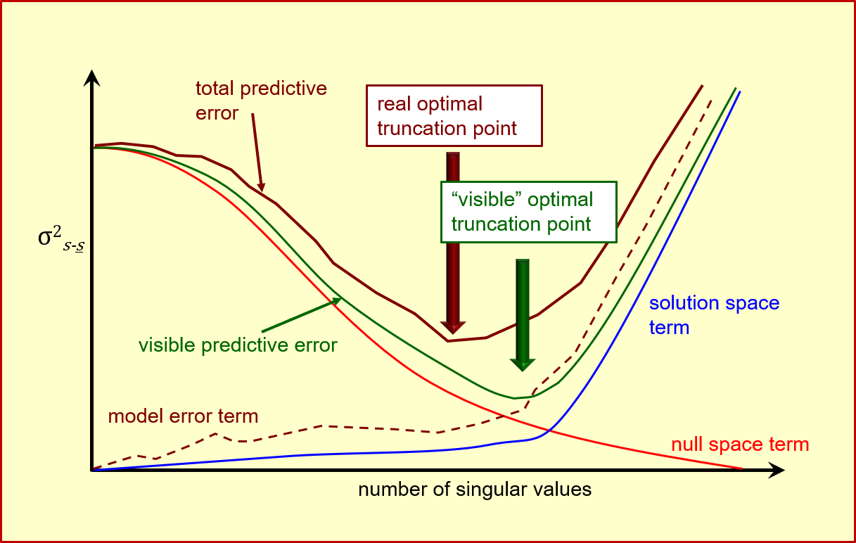
The effects of model defects on predictive error variance.