Bayes equation links prior parameter uncertainties to posterior parameter uncertainties. So to calculate posterior uncertainties, we must provide prior uncertainties.

Well - not quite.

If model parameters are uniquely estimable using field measurements (that is, if an inverse problem is well-posed), then prior parameter uncertainties do not matter so much. The same applies to certain predictions. If a prediction is sensitive only to combinations of parameters that are informed by measurements (that is, if it is sensitive to combinations of parameters that lie within the calibration solution space while being insensitive to combinations of parameters that line within the calibration null space), then prior parameter uncertainties matter little as far as that prediction is concerned.

Back to Bayes equation.

Let's make some assumptions. Let us assume the following.

•Prior parameter uncertainties can be characterised using a multi-normal distribution. Let C(k) be the covariance matrix associated with this distribution. (k is the vector of model parameters.)

•Noise associated with field measurements can be characterised using another multi-normal distribution. Let C(ε) be the covariance matrix of measurement noise. (ε is the vector of measurement noise.)

•The model is linear. That is, the relationship between model outputs and parameters can be described by a matrix. This is the sensitivity (i.e. Jacobian) matrix J.

Under these circumstances, it can be shown that either of the following equivalent matrix equations (derived from Bayes equation) can be used to calculate the posterior covariance matrix C'(k) from the prior covariance matrix C(k).

C'(k) = [JTC-1(ε)J + C-1(k)]-1

C'(k) = C(k) - C(k)JT[JC(k)JT + C(ε)]-1JC(k)

The second equation makes it clear that history matching reduces uncertainty.

The PREDUNC7 utility (supplied with PEST) uses either of these equations (its your choice) to calculate a posterior covariance matrix from a prior covariance matrix. From the above equations, it is apparent that this utility (and many other linear analysis utilities supplied with PEST) require three matrices. These are the C(k), C(ε) and J matrices.

A J matrix resides in a Jacobian matrix file (i.e. a JCO file) that complements a PEST control file. Prior parameter uncertainties are provided in a parameter uncertainty file. The contents of the C(ε) matrix are obtained from a PEST control file.

We now discuss how these matrices are obtained in greater detail.

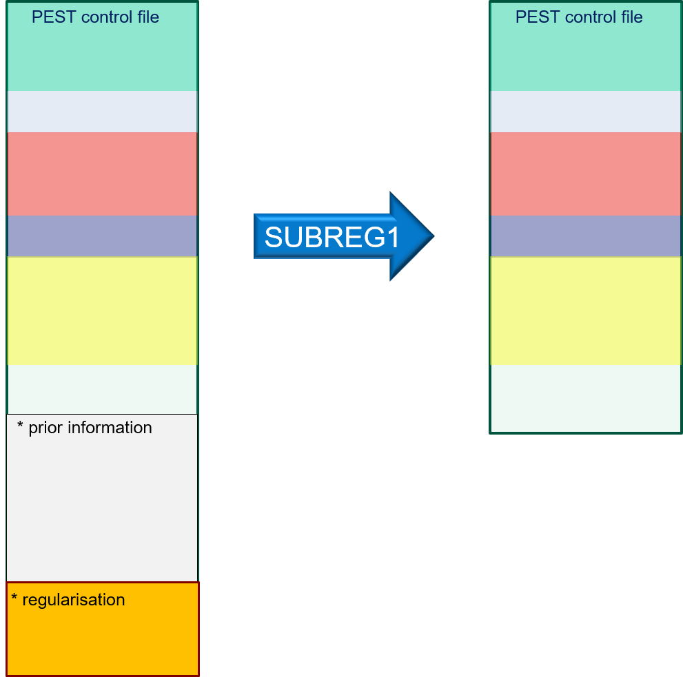
Production of a Jacobian matrix file (i.e. JCO file) requires that you run PEST, normally with the NOPTMAX control variable set to -1 or -2 and with optimised parameter values as initial parameter values. Remove regularisation from this file before calculating this matrix. Alternatively, if you have already produced a JCO file based on a PEST control file that contains regularisation, remove regularisation from the PEST control file using the SUBREG1 utility, and then run JCO2JCO to obtain a new JCO file.

Most of the uncertainty analysis utilities that are supplied with PEST assume that the covariance matrix of measurement noise C(ε) is diagonal. That is, they assume that the noise associated with each measurement is statistically independent of the noise associated with all other measurements.

Often this is not quite true. If structural noise is taken into account, then it is definitely not true. However we never know the covariance matrix of structural noise. Furthermore, in most (but not all) incidences of groundwater model deployment, uncertainty is dominated by nonuniqueness rather than by measurement noise. So approximations that are made in filling of the C(ε) matrix do not matter too much.

PEST linear analysis utilities obtain measurement noise from weights that reside in a PEST control file. They assume that each weight is inversely proportional to the inverse of the standard deviation of measurement noise that is associated with each measurement, and that this proportionality constant is the same for all measurements. All utilities ask, in one way or another, what this proportionality constant is.

The easiest answer to this question is "1.0". You can provide this answer when all weights are "correct". Weights are correct when the measurement objective function for the calibrated model is equal to the number of non-zero-weighted observations. The reason for this is easy to work out. If each weight is the inverse of the standard deviation of noise that is associated with its respective measurement, then the average squared weighted residual is 1.0. Multiply this by the number of observations to obtain the objective function.

The PWTADJ2 utility that is supplied with the PEST suite can create a PEST control file in which weights are correct.

So, after calibrating a model, do the following.

1.Use the PARREP utility to insert optimised parameter values into a new PEST control file.

2.Use the SUBREG1 utility to remove regularisation from this file.

3.Set NOPTMAX to -1 or -2.

4.Run PEST to calculate the objective function and a Jacobian matrix.

5.Use the PWTADJ2 utility to build a new PEST control file. In this new PEST control file the objective function for each parameter group will be equal to the number of observations in the group.

6.Run JCO2JCO to obtain a Jacobian matrix for this new PEST control file.

This final PEST control file can be used as a basis for linear parameter and predictive uncertainty analysis. Weights are "correct". And it has a complimentary Jacobian matrix.

Some linear analysis utilities ask for the "reference variance". This is the ratio of the objective function to the number of non-zero-weighted observations. Obviously, if weights are correct, the reference variance is 1.0. Other utilities ask for the factor by which weights must be adjusted to make them correct. Obviously, if weights are correct this ratio is 1.0.

Use of the PWTADJ2 utility prior to embarking on parameter or predictive uncertainty analysis is therefore recommended. It makes things less complicated.

A moment's reflection

Before describing a parameter uncertainty file, the contrast between regularisation and uncertainty analysis is worth a few moment's reflection. Both of these use covariance matrix files to describe the prior uncertainties of subsets of parameters.

Regularisation powers a history-matching process that informs us of the heterogeneity that must exist to explain measurements of system behaviour. In contrast, uncertainty analysis explores the heterogeneity that may exist that is compatible with measurements of system behaviour. The same prior parameter covariance matrix may be used in both processes. But it is used for different reasons. When undertaking regularised inversion, it dictates the patterns that minimally emergent heterogeneity must adopt. When undertaking uncertainty analysis, it dictates the patterns that random realisations of heterogeneity can adopt.

Prior parameter uncertainty

Before doing any kind of uncertainty analysis - linear or nonlinear - a parameter uncertainty file must be prepared. This is normally used to express prior parameter uncertainties. However it can be used to express posterior parameter uncertainties as well.

The format of a parameter uncertainty file is described in Part 2 of the PEST manual. An example is shown below.

As is apparent from the above figure, a parameter uncertainty file is subdivided into sections. Sections can be of two types, namely STANDARD_DEVIATION and COVARIANCE_MATRIX.

Here is a particularly important point. If a parameter is designated as log-transformed in a PEST control file, then uncertainties that are provided in the uncertainty file must pertain to the log of that parameter.

If a parameter is not correlated with another parameter, then its prior uncertainty can be expressed using its standard deviation. If you are unsure what this is, then divide the difference between its upper and lower bounds by 4 (assuming that these bounds mean something). If the parameter is log-transformed, then you will need to divide the difference between the logs of its upper and lower bounds by 4.

The PPCOV, PPCOV3D, PPCOV_SVA and PPCOV3D_SVA utilities supplied with the groundwater utilities can be used to build covariance matrices for subsets of spatially-distributed parameters (for example pilot point parameters). The lines within each COVARIANCE_MATRIX block of a parameter uncertainty file that follow the name of a covariance matrix file inform programs which read this file how to relate rows and columns of the covariance matrix to parameters which are listed in the "parameter data" section of the PEST control file. See PEST documentation for further details.

The PREDUNC family is supplied with the PEST suite. Most members of this utility family calculate predictive uncertainty rather than parameter uncertainty. However PREDUNC7 calculates parameter uncertainty.

PREDUNC7 writes a parameter uncertainty file that contains only one block. This block is a COVARIANCE_MATRIX block. PREDUNC7 also writes the covariance matrix file that is cited in this block. This file contains the posterior parameter covariance matrix.

Where parameter numbers are large, the posterior parameter covariance matrix file is huge. (It contains NPAR*NPAR elements where NPAR is the number of adjustable parameters.) Posterior parameter variances occupy the diagonal elements of this file. Variance is the square of standard deviation.

The diagonal of this matrix can be extracted using the MATDIAG utility (supplied with PEST). MATDIAG records the diagonal as a vector in PEST matrix file format. Variances occupy the first part of this file, while parameter names occupy the second part of this file. Use a text editor with column-cut-and-paste functionality to place parameter names and values alongside each other. Then import the table into a spreadsheet. Once in a spreadsheet, you can take the square root of posterior variances to obtain posterior standard deviations.

As is discussed above, it is a modeller's responsibility to place prior parameter uncertainties into a parameter uncertainty file before undertaking any kind of (linear or nonlinear) uncertainty analysis. Sometimes, however, it is nice to have these uncertainties listed in a single column rather than being distributed between STANDARD_DEVIATION and COVARIANCE_MATRIX blocks. An easy way to do this is to fool PREDUNC7 into calculating "posterior parameter uncertainties" that are actually prior parameter uncertainties. Then you can follow the procedure that is outlined in the previous section to import prior parameter variances into a spreadsheet, and calculate prior standard deviations.

In your PEST control file, set all weights that are not zero to a very low value, for example 1.0E-30. This implies that the level of measurement noise is so high as to render the observation dataset worthless. Then run PREDUNC7 in the way described above to obtain a "posterior" parameter covariance matrix file which is really a prior parameter covariance matrix file.

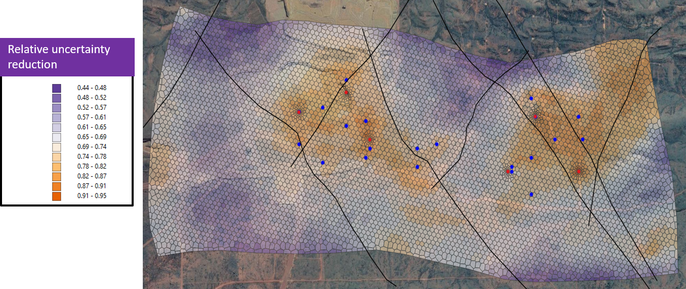
Maps of posterior parameter uncertainty, or of related quantities such as ratio of posterior to prior parameter standard deviations, are often very informative components of a modelling report. Here are some steps that you can follow to help you produce these kinds of maps.

In the batch or script file that PEST runs when it calibrates the model, a simulator (such as MODFLOW) is normally preceded by a preprocessor that fills model input files using parameter values that are adjusted by PEST. Parameters may be assigned to zones, pilot points and/or other parameterisation devices that are supported by packages such as PLPROC. PLPROC, as a model preprocessor, undertakes spatial interpolation of these values to the model grid, and then writes model input files.

Most modellers have software that can import model input files into a GIS or other package where hydraulic property values can be contoured or shaded on a map background. This same software can be used to contour and shade spatially-varying quantities that describe prior or posterior parameter uncertainty (or their ratios) if you follow these steps.

1.Using a text editor, place the parameter-related quantity that you want to plot into a parameter value file. In this file, a value is assigned to every parameter. Let's assume that these values characterise posterior parameter standard deviations.

2.Run the PARREP utility to place these standard deviations into a PEST control file as initial parameter values.

3.Set NOPTMAX to 0 in this file, and run PEST.

The model will probably crash. (If it does not crash, stop it yourself by pressing <Ctl-C>.) Meanwhile model input files will have been filled with spatially interpolated values of parameter standard deviations. Import these into your GIS and plot them as if they were hydraulic property values.

The following picture is extracted from a GMDSI worked example report.