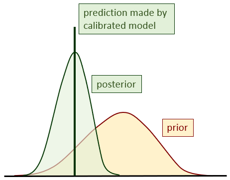
An infinite number of parameter sets can usually be found that allow model outputs to fit field measurements of system behaviour. Furthermore, the greater the hydraulic property detail that these parameters represent, the greater is their number, and the greater is their post-history-matching nonuniqueness.

So why seek uniqueness at all? And what does "uniqueness" even mean under these circumstances?

It can be shown mathematically that, provided certain conditions are met, it is possible to find a set of model parameters that have a special property. This property is that all predictions made by the model lie at the centres of their respective posterior probability distributions.

There are other ways of saying this. We can say that this special set of parameters minimises the posterior error variance of all model predictions. That is, they minimise the potential for predictive wrongness. This is not to say that the potential for wrongness of some model predictions is not large. This depends on the prediction, and on the information content of the calibration dataset as it pertains to that prediction. Minimisation of the potential for predictive wrongness is achieved by ensuring that this potential is symmetrical with respect to the prediction.

It can also be shown that the parameter set which achieves this status is unique.

So uniqueness is possible. And uniqueness can be useful. But "unique" does not mean "correct".

The situation is depicted below.

If it is decided that groundwater management will be based on a single parameter set, then it is obvious that this parameter set should be determined through model calibration. It is also obvious that calibration should attempt to achieve the goals that are outlined above. That is, it should attempt to guarantee a status of minimum error variance for all predictions made by the calibrated model.

In practice, this ambitious goal may not be achieved. Sometimes calibration can induce parameter bias. Parameter bias may (or may not) induce predictive bias; this depends on the prediction. In general, the greater the extent to which a prediction of future system behaviour is informed by measurements of its past system behaviour, the less does parameter bias translate to predictive bias. Under these circumstances, all that is required of the decision-support modelling process is that the model replicate the past well. Model calibration then becomes a form of machine learning.

However the opposite is the case for other predictions. Calibration of a defective simulator can force parameters to adopt compensatory roles as the model is history-matched. Predictions that are partly informed by these parameters and partly informed by null space parameter combinations may then be biased. Model defects that can provoke calibration-induced bias of some model predictions include omission or poor numerical representation of certain processes or boundary conditions, and use of parameterisation devices such as zones of piecewise constancy which do not reflect the penchant for hydrogeological heterogeneity that prevails in the subsurface.

It may not be possible to build a model that can guarantee absence of bias in all predictions. It follows that model design, and the model calibration process, may need to be prediction-specific. Problem decomposition is as important as ever. But that is not our concern for now. Our concern is the pursuit of uniqueness.

First, some terminology.

When we provide a set of parameter values to a model, and then use the model to calculate system states and fluxes, we solve a "forward problem". In contrast, if we try to infer model parameters from measurements of system state and flux, we solve an "inverse problem".

Intuition and mathematics readily inform us that our ability to infer system hydraulic properties (especially system hydraulic property detail) diminishes with the number of measurements that we have at our disposal. This is because many sets of parameters allow a model to replicate a limited set of field measurements. Where the solution to an inverse problem is nonunique, the inverse problem is said to be ill-posed.

As is described above, uniqueness (which is to be distinguished from correctness), can nevertheless be attained. Furthermore, it can be attained in a way that serves the decision-making process well (as long as predictive bias is avoided). The means through which an ill-posed inverse problem is turned into a well-posed inverse problem is termed "regularisation".

Hence model calibration is, in essence, the pursuit of a regularised solution to an ill-posed inverse problem.

Regularisation methodologies fall into three broad categories. These are:

•manual;

•subspace;

•Tikhonov.

Each has advantages and disadvantages. In groundwater modelling we generally use all three.