It is because we know so little about so much when it comes to characterisation of groundwater systems.

We know the partial differential equation that groundwater flow obeys (except where porosity is cavernous). This is based on conservation of mass and Darcy's law. But here are some of the things that we do not exactly know:

•the subsurface disposition of different rock types;

•the hydraulic properties of the rocks and sediments through which water flows, and whether processes of rock formation, diagenesis, metamorphism, tectonics and weathering have introduced preferential flow paths to these rocks;

•the degree to which groundwater and surface water bodies interact;

•the areal and temporal distribution of recharge;

•the connectedness of a studied groundwater system with neighbouring systems;

•historical (and sometimes present-day) pumping from the system.

Matters become even more difficult when the need for hydraulic property upscaling is taken into account.

In the old days, construction of a groundwater model rested on a suite of assumptions concerning many of the items listed above. It was assumed that these assumptions could not be so wrong as to "invalidate" model predictions. This is despite the fact that groundwater models were (and still are) often structurally complex, and include many structural details (requiring assumptions about assumptions) so that they can resemble "the real thing". In order to make people feel better about the model's utility as a decision-making tool, values of some its features were back-calculated from history-matching. That is, the model was "calibrated".

Usually, calibration was preceded by definition of a number of broad zones in which hydraulic properties were deemed to be spatially invariant. "The fewer parameters the better" was the calibration mantra. By adjusting some of the hydraulic properties ascribed to these zones, a level of model-to-measurement fit was attained which was inevitably deemed to be "satisfactory". The model was then "licensed to predict".

Licensed to predict (like 007 is licensed to kill).

If predictive uncertainty was acknowledged, it was "measured" by varying the values assigned to zone-based hydraulic properties until model-to-measurement misfit was considered to be unsatisfactory. Changes in model predictions incurred by this process were deemed to be a measure of their uncertainty.

In some cases a small number of alternative models were built instead of a single model. Each of these was based on a different conceptual model. Each was parameterised and calibrated in the same way. Predictive uncertainty was then "measured" as contrasts between model predictions between the calibrated models.

Is this the best way to handle uncertainty? In environmental modelling, there is no right or wrong. However there are metrics which make sense. In our opinion this approach to decision-support modelling is rather cumbersome. It has little theoretical basis. It does little to realise the abductive potential of modelling. Nor can it generally provide protection against decision-support modelling failure.

The use of broad zones of assumed hydraulic property constancy may avoid calibration nonuniqueness. However sweeping nonuniqueness under the carpet sweeps uncertainty under the carpet. This is because calibration nonuniqueness (or "equifinality" as it is sometimes called) is a major contributor to predictive uncertainty. In many cases it exceeds uncertainties that arise from conceptual model differences.

Furthermore, if modellers and stakeholders are prepared to sacrifice "picture perfect" for a little model abstraction, then it may be possible to represent conceptual differences using adjustable parameters. (Not that zones of piecewise constancy has any resemblance to "picture perfect".) Methods that are discussed in these pages (and in many textbooks on uncertainty quantification) can then be used to examine the effects of conceptual nonuniqueness on predictive uncertainty.

Where a model's construction and parameterisation rests on assumptions, any predictions and associated uncertainties that are examined using that model are conditional on the correctness of these assumptions. If a prediction is conditional on something whose potential wrongness is not examined, then it may be biased by an unknown amount. (Think of "bias" as unquantifiable uncertainty.)

At the other end of the modelling spectrum is probabilistic representation of any aspect of model construction and subsurface hydraulic properties that are incompletely known. For the moment, let us define a "parameter" as any aspect of a model that has fluid representation. It is therefore adjustable - either to express its uncertainty or to improve model-to-measurement fit. So full recognition of uncertainty requires that just about all aspects of a model's design become adjustable.

This approach to model design may indeed be conceptually "pure", given our incomplete knowledge of natural systems. However it is accompanied by severe practical difficulties. A numerical model requires a grid (so that matrix equations based on partial differential equations can be formulated and solved). Construction of a grid requires certain assumptions. Programmed into most numerical model boundary conditions are simplifying assumptions of the system's interaction with external processes. Assumptions cannot be avoided, for without some assumptions there is no model.

Despite all of these problems, model construction under the premise that "if you don't know the value of something then let it wiggle" is less numerically intractable than it used to be. This is thanks to the advent of ensemble methods. To be sure, ensemble methods come with their own set of assumptions. Indeed, the concept of "let it wiggle" implies a probability distribution. This, in turn, requires that assumptions be made about hydraulic property spatial correlation and connectedness, together with assumptions about the regions over which these assumptions apply.

There will always be assumptions. However the more that unknown aspects of a natural system can be represented fluidly rather than rigidly, the less does quantifiable uncertainty become unquantifiable bias.  

Suppose that you are building a model in an area where there are no measurements of system state available. That is, you have access to no measurements of borehole heads, and no measurements of flow into or out of system boundaries. Suppose that you are trying to embrace uncertainty by representing all uncertain aspects of the modelled system stochastically. "Stochastic representation" can take many forms. You may sample many different realisations of uncertain hydraulic properties and/or system stresses from respective probability distributions. Or, depending on your approach to uncertainty analysis, you may represent these probability distributions mathematically. In either case, a probability distribution is required. This is referred to as the "prior probability distribution". It represents all that you know about the investigated system. At the same time, it represents all that you do NOT know about the investigated system.

Suppose now that measurements of system state become available. Obviously, a model which cannot reproduce the measured past of a system cannot be asked to predict its future. However, a model's capacity to replicate measurements of system state and flux here and there does not eliminate parameter (and therefore predictive) uncertainty. It will, however, constrain the model's overall parameter probability distribution. This modified probability distribution of model parameters is referred to as the "posterior parameter probability distribution".

The constraining effect of history-matching is described by Bayes equation. Let us use the term P(k) to denote the prior probability distribution of parameters. P() stands for "probability" and k represents parameters. k is bold because it is a vector. (It is a vector because there are lots of parameters.) We use the vector h to denote the set of measurements of system behaviour that the model must replicate. It is also a vector. We use the term P(k|h) to denote the posterior probability distribution of parameters. This is the probability distribution of parameters conditional on h (that is what "k|h" means). Bayes equation can then be written as follows.

P(k|h) ∝ P(h|k)P(k)

The first term on the right of Bayes equation is the likelihood function. It increases to the extent that model outputs match field data. Its exact value is determined by the amount of noise that is associated with field measurements, and by the statistics of this noise. So this, too, is a stochastic quantity. The realisation of measurement noise that accompanies any field measurement is unknown. However if its statistical properties are known, or can be guessed (another assumption), then the likelihood function can be formulated.

You can look at Bayes equation in a number of ways. Perhaps the easiest way to view it is as a kind of filter.

As stated above, the prior distribution of model parameters encapsulates our expert knowledge. The fact that a probability distribution is required to encapsulate our knowledge says a lot about our knowledge. It says that we do not know the details of a groundwater system. But we do know something about the shapes, dispositions and connectedness of the details. Dispositions and connectedness are very important to groundwater flow.

Unfortunately, while the concept of a probability distribution allows us to express the fact that we know something, but not everything, it is often hard to express this type of knowledge mathematically (particularly as it applies to subsurface systems). So we just do our best. For the moment, let us summarise the status of our prior knowledge by admitting that we do not know what is under the ground. But we are pretty sure of what is NOT under the ground.

However not just any picture of the subsurface that our P(k) allows us to conjure up can be used in a model that is intended to predict the future behaviour of a system. These pictures must be limited to those that allow the model to replicate measurements of its past behaviour to within a margin set by noise associated with those measurements. P(h|k) is therefore a type filter that P(k) must pass through before it becomes P(k|h).

There are various ways to do this filtering operation. Depending on the assumptions that we make, some of them are easy. However, with fewer assumptions, the numerical difficulty of this filtering operation rises rapidly.

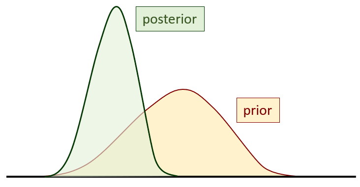
If the uncertainties of model parameters are reduced through history-matching, then the uncertainties of model predictions must also be reduced. Right?

Unfortunately not. It depends on the prediction. Measurements of certain types of system behaviour at certain times and at certain places will constrain the uncertainties of some parameters. (More accurately, they will constrain the uncertainties associated with some combinations of parameters). However management-critical predictions may not be sensitive to these parameters. So history-matching may do little to constrain the uncertainties of these predictions.

In general, the greater is the sensitivity of a prediction to parameterisation detail, the less is its uncertainty likely to be reduced through history-matching. Examples of detail-dependent predictions include contaminant fate, and the response of a system to extreme climatic events - especially those which are more extreme than it has experienced in the past. A good rule of thumb is that the greater resemblance that a prediction bears to historical measurements (in type, location and system stress regime), the more likely it is that its uncertainty is reduced through history matching.

The ideal situation is shown below. See how the posterior probability distribution of the prediction is narrower than its prior probability distribution. At the same time, the probability density function is taller. This is because all probability distributions must integrate to unity.

Prior and posterior predictive probability distributions.

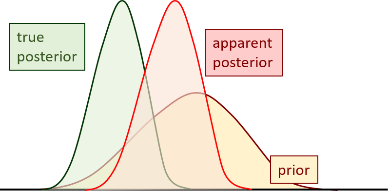
It all sounds so simple. After all, Bayes equation is an elegant way of stating the obvious.

But environmental modelling is not simple. We cannot capture much of reality on a computer - neither as a picture nor as a probability distribution.

Models are replete with assumptions and simplifications. Sometimes these assumptions are wrong; sometimes these simplifications are a poor representation of subsurface reality. This may not prevent us from attaining a very good fit between model outputs and field measurements. However in doing this, model parameters may compensate for aspects of the model that are wrong. That is, they may adopt surrogate roles.

Does this matter? If we can fit the calibration dataset well, have not model defects been "calibrated out"?

This is complicated - more complicated than can be described by Bayes equation. Furthermore, it depends on the prediction. For predictions that are similar to measurements against which the model has been history-matched, a good fit with the past ensures a good fit with the future, regardless of model imperfections. (Modelling becomes like machine learning.) For other predictions, the opposite is the case. History-matching may actually bias these predictions. And remember, bias cannot be quantified.

So what is good for one prediction, may not be good for another. Given that all models, no matter how complex they are, are full of defects, this suggests that model construction and deployment may need to be prediction specific. The allure of "simulation integrity" is further away than ever.

When an imperfect model is history-matched, some predictions may incur bias.