Because integrity of the Jacobian matrix is fundamental to correct and efficient solution of an inverse problem, PEST provides a plethora of options for derivatives calculation.

PEST (but not PEST_HP) allows a model to calculate some or all of the sensitivity matrix (i.e. the Jacobian matrix) itself. Access to this option is available through the JACFILE control variable in the "control data" section of the PEST control file. If a model can calculate derivatives quickly, inversion time may be greatly reduced.

Mostly, however, derivatives must be calculated using finite parameter differences. Options for doing this are many. They are accessible through the "parameter groups" section of a PEST control file. We discuss a few of them here, and simply inform you of the existence of the others.

An interesting option that we do not discuss here is PEST's (and PEST_HP's) ability to use different model commands when calculating derivatives with respect to different parameters. This is invoked through the NUMCOM control variable . Companion functionality (observation re-referencing) is available through the OBSREREF control variable. Both of these variables can be found in the "control data" section of a PEST control file.

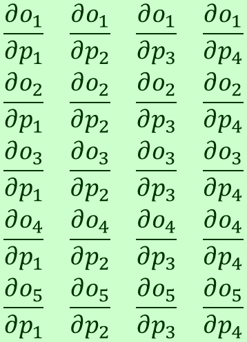
At the heart of the Gauss-Marquardt-Levenberg method that is used by PEST to estimate parameters is a sensitivity matrix (i.e. a Jacobian matrix). This is a matrix of partial derivatives of model outputs with respect to parameters.

A Jacobian matrix.

While other parameter estimation methods that do not require a Jacobian matrix (such as those supported by the SCEUA_P and CMAES_P global optimisers) are sometimes deployed, their use becomes numerically impossible for estimation of more than a few parameters. Even ensemble methods such as that implemented by PESTPP-IES use a Jacobian matrix; they calculate a rank-deficient approximation to this matrix.

As is described below, PEST calculates derivatives of model outputs with respect to parameters using finite differences. Many options are available to tune calculation of finite-difference derivatives to the numerical circumstances that a modeller faces. However, in the end, none of these will work well if numbers calculated by a model are numerically corrupted.

Numerical corruption can arise in many ways. Older versions of MODFLOW were plagued by problems associated with dry cells. The MODFLOW SFR package can face numerical challenges if streams stop flowing. In general, the more nonlinear is the problem that a simulator must solve, the greater are the chances that it will encounter numerical difficulties. These may express themselves as solution non-convergence as parameters are upgraded, and deterioration in the quality of finite differences as parameters are varied incrementally.

It makes sense to avoid use of troublesome simulation functionality unless it is absolutely essential to the decision-support role that modelling must serve.

There are a few basic steps that you can take (that have nothing to do with PEST) that can improve the integrity of finite-difference derivatives calculation a great deal - enough to make the difference between PEST being able to calibrate your model or not.

Model output files

Make sure that model-generated numbers that PEST must read are recorded on model output files with a high level of numerical precision - at least seven significant figures if the model allows it. When differences are taken between numbers that are close together, the first few significant figures are lost from the difference. So all useable information resides in the last few significant figures. If they are missing, then the difference is either zero, or greatly in error.

Communication between model components

More often than not, a model is comprised of more than one executable program. These model components communicate with each other using files. Make sure that the numbers that one model component passes to another are recorded with maximum precision. This is most easily achieved if they communicate using binary files. Under these circumstances submodel-to-submodel communication suffers no loss of precision at all.

Solver convergence criteria

Many simulators solve large matrix equations using iterative solvers. Set the convergence criteria on these solvers tighter than you normally would. For example, a setting of 1.0E-3 for the MODFLOW HCLOSE heads closure criterion is often fine if all that you want to do is calculate heads. However HCLOSE should be set to 1.0E-4 (or less) if derivatives of heads with respect to MODFLOW parameters must be calculated. This is especially the case when using parameterisation devices like pilot points. There are many advantages to be gained from highly-parameterised inversion. However the sensitivity of each individual parameter falls as the number of parameters grows.

Variables that appear in the "parameter groups" section of a PEST control file are shown below. One line is required for each parameter group. Some variables on each line are mandatory, while others are optional.

The first variable (PARGPNME) on each line of the "parameter groups" section of a PEST control file is the name of a parameter group. All parameters that are listed in the "parameter data" section of a PEST control file must be assigned to one of the parameter groups that are listed in the "parameter groups" section of the PEST control file. Parameter group names can be 12 characters or less in length (up to 200 characters for PEST++). However it is a good idea to confine their length to 6 characters. This allows the ADDREG1, ADDREG2 and ADDREG3 utilities to form prior information group names from parameter group names by appending "regul_" to the beginning of the parameter group name. The "regul_" prefix allows PEST to distinguish regularisation observations and prior information equations from other observations and prior information equations.

Part of the "parameter groups" section of a PEST control file is shown below. Note that on most occasions of PEST usage, the SPLITTHRESH, SPLITRELDIFF and SPLITACTION control variables are omitted from this section, and so are not shown below. However if a model is behaving badly, then use of these variables can reap great rewards.

Read the PEST manual in order to learn the role that each of these variables play. Here we describe the principles of finite-difference derivatives calculation, and provide some advice on which options to choose.

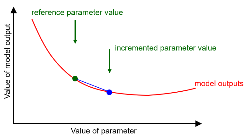
General

Finite difference derivatives can be calculated using 2, 3 or 5 parameter and model output pairs. The integrity of the approximated derivative increases with the number of pairs that are used. So does the number of model runs.

For all of these options "reference model outputs" are available from the previous iteration. These are values of model-calculated observations calculated using best parameter values that were achieved during that iteration. So to calculate derivatives based on 2, 3 or 5 pairs, then 1, 2 or 4 model runs are required per parameter. (Note that PEST allows derivatives to be calculated differently for different parameter groups.)

Two-point derivatives

Use of two points is easy to understand and easy to implement.

Vary each parameter by a small amount and run the model. The difference in values calculated for a particular model output divided by the parameter increment is an approximation to the derivative. That is, the slope of the chord is adopted as an approximation to the tangent at the reference point.

The slope of the chord is easy to calculate, and requires only one model run. The problem is that the chord extends from the reference point in only one direction. If the relationship between the model output and the value of the parameter is curved, then the chord approximation is slightly wrong.

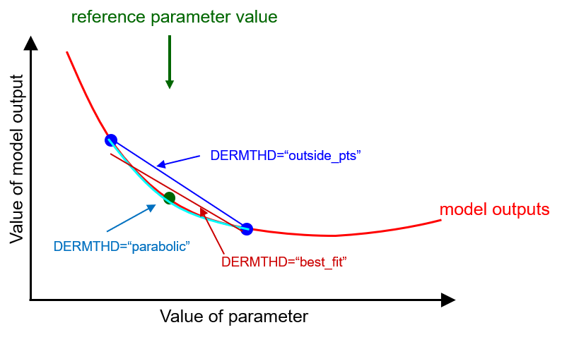
Two-point finite-difference calculation of a derivative.

So how large should the increment be? If it is too large, the chord is not a good approximation to the tangent. If it is too small, then the differencing of two numbers that are close to each other incurs numerical errors. (This is especially the case if model outputs are written to their files with limited precision, or if a numerical model has an iterative solver that does not converge properly.) Generally an increment value of 1% to 2% of the parameter's current value works well. But you may want to instruct PEST to place an absolute lower bound on this increment. In general, the more granular are model outputs (i.e. the more numerically noisy are model outputs), the larger should the parameter increment be.

Increment lengths are set using the INCTYPE, DERINC and DERINCLB control variables.

Three-point derivatives

This is sometimes referred to as "central derivatives".

The model is run twice - once with a parameter incremented and once with the parameter decremented. Three options are available for calculation of an approximation to the derivative using these three points (i.e. the incremented/decremented points and the reference point). The option is chosen using the DERMTHD variable. "Parabolic" is the best option if the model is well-behaved. If its outputs are somewhat granular, "outside_pts" may be better.

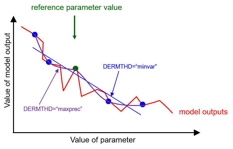
Three-point finite-difference calculation of a derivative.

Five-point derivatives

This option is expensive as it requires four model runs. It should only be chosen if model outputs are really dirty. Under these conditions, there may be better options, for example split-slope analysis.

Once the four model runs have been completed, the DERMTHD "minvar" option is probably the safest. After all, you would not have asked the model to do these four model runs unless there was a good reason. And the good reason is to suppress model numerical noise.

Five-point finite-difference calculation of a derivative.

Switching from one to the other

Experience has demonstrated again and again that the most efficient derivatives calculation strategy is to start off with two-point derivatives calculation and then switch to three-point derivatives calculation when the extra accuracy is required. Set the FORCEN derivatives control variable to "switch" to implement this option. PEST makes the switch to three-point derivatives calculation when the objective function fails to fall by a user-prescribed relative amount. This amount is set by the value of the PHIREDSWH variable. The PHIREDSWH variable resides in the "control data" section of the PEST control file. A setting of 0.1 works well.

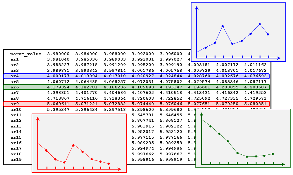
If PEST is unable to lower the objective function (which measures model-to-measurement misfit), or does not lower it as much as you think that it should, then the reason is probably lack of integrity of finite-difference derivatives. (This is provided that singular value decomposition or LSQR is implemented by PEST so that inverse problem ill-posedness does not present a numerical problem.)

The JACTEST and JACTEST_HP utilities (that are supplied with PEST and PEST_HP respectively) can be used to test the integrity of finite difference derivatives calculation. Each of these programs reads a PEST control file. It then varies the value of a user-specified parameter in incremental amounts, both up and down from its initial value as specified in the PEST control file. Model-calculated observation values for all of these parameter values are recorded on an output file which is easily imported into a spreadsheet for further analysis.

In many cases you will be surprised at what you see. Model numerical nuances may artificially reverse derivatives at certain parameter values. At best, this makes PEST's work difficult. At worst it creates artificial local optima.

JACTEST can expose non-differentiability of model outputs with respect to parameters.

The POSTJACTEST utility that is supplied with PEST reads a JACTEST output file. Where there are many observations, this output file can be large. POSTJACTEST finds model outputs for which derivatives appear to be most corrupted.

Calculation of three-point derivatives provides PEST with an opportunity to assess the integrity of derivatives calculation, and to possibly take some evasive action. Recall that when undertaking three-point (sometimes called central) derivatives calculation, PEST increments and then decrements a parameter. It then calculates an approximation to the derivative using the three model outputs that correspond to the reference and incremented/decremented parameters.

Using the optional SPLITTHRESH, SPLITRELDIFF and SPLITACTION control variables that appear in the "parameter groups" section of a PEST control file, you can ask PEST to do more than this. You can ask PEST to compare the individual slopes calculated in both the forward and backward directions from the reference parameter value. If these are very different (and particularly if the slopes are opposite), this indicates that something is wrong. Depending on the setting of the SPLITACTION control variable, PEST then takes remedial action.  Options are:

•set the derivative to zero;

•use the smaller of the two individual slopes (under the assumption that the larger one is in error);

•use the derivative from the previous iteration.

Experience has demonstrated that this simple procedure can sometimes work very well.

Sometimes a model has a strong negative reaction to a certain set of parameters. It calculates stupid model outputs. If this happens in response to a set of upgraded parameters, the objective function that PEST calculates from model outputs demonstrates the model's distaste for them. PEST tries another set of parameters.

However if this happens during finite-difference filling of the Jacobian matrix, the result will be disastrous. PEST does not calculate an objective function following every model run that is used for derivatives calculation. What happens, however, is that the difference in model outputs between reference parameters and an incrementally varied individual parameter is huge. The derivative is therefore enormous. This messes up the inversion process. PEST "sees" only one "extremely sensitive" parameter, and ignores the others.  The whole iteration is wasted.

PEST_HP provides two optional control variables named JCOWARNTHRESH and JCOZEROTHRESH that can address this situation. These must be provided in the "control data" section of the PEST control file. See the PEST_HP manual for placement details.

JCOWARNTHRESH has a default setting of 1.0E30. (This is very conservative.) PEST_HP writes a warning to the screen and to its run record file if the sensitivity of any parameter is above this threshold.

An appropriate setting for JCOZEROTHRESH can eliminate objectionable sensitivities with respect to offending parameters by replacing them with zero. The default value for JCOZEROTHRESH is zero. This tells PEST to ignore outrageous sensitivities. Set JCOZEROTHRESH to an appropriate value yourself if you wish to shield the inversion process from this problem.

Courtesy of BOM.

PEST_HP allows a modeller to use realisations of random parameter increments instead of individual parameter increments when filling a Jacobian matrix. The number of realisations that comprise an ensemble can be far fewer than the number of parameters that require estimation. Use of increment realisations to calculate an approximate, rank-deficient Jacobian matrix can increase the model-run efficiency of an inversion process enormously.

See the PEST_HP manual for further details.