Before we discuss subspace methods and Tikhonov regularisation, let's spend a few moments talking about benefits that accrue from using lots of parameters. But first, let's briefly address the subject of appropriate model complexity. For a far more complete discussion of this topic, see the GMDSI monograph.

Decision-making is a broad field of study. Here we make a simple, but obvious, point.

The making of a decision requires an analysis of what can go wrong if a certain course of action is adopted. It follows that decision-support modelling assists environmental management if it can illuminate the possibility of unwanted outcomes of a contemplated management strategy. Targeted predictive uncertainty analysis is fundamental to this. The integrity of uncertainty analysis rests, in turn, on representation within a model of aspects of system behaviour or heterogeneity that may precipitate unwanted management outcomes. Whether the parameters that govern these processes and potential heterogeneity are estimable or not is beside the point. It is their pertinence to a prediction of management interest that matters. Nonuniqeness will engender uncertainty. It is through analysis of uncertainty that decision-makers become aware of what can go wrong.

In days gone by, modellers were strongly advised to err on the side of parameterisation simplicity, thereby avoiding problems associated with parameter nonuniqueness and/or model-to-measurement overfitting. These days are over. If parameters cannot be uniquely estimated, and if the need for predictive uncertainty analysis is taken seriously, then the nonuniqueness of parameters constitutes the most powerful reason for their retention in a model. This is a reversal of the old ways of thinking.

Parameter nonuniqueness is not a problem. It can be handled numerically with ease. At the same time, there is no reason that use of a large number of parameters will result in model-to-measurement over-fitting; this too is easily avoided.

However, the focus of the present section is on calibration, and not on uncertainty analysis. So how does working in a highly parameterised environment assist model calibration?

Remember what calibration is intended to achieve. It is intended to endow a model with the ability to make predictions whose potential for error is minimised. This requires that parameters not be required to compensate for disinformation that is hardwired into their design as they are adjusted to improve model-to-measurement fit. This, in turn, requires that if the inversion process requires that parameter heterogeneity be introduced to the model domain, then there should be:

•no obstacles to where that heterogeneity is introduced, and

•an encouragement for heterogeneity to arise in ways that are geologically plausible while not preventing its emergence in other ways if this is necessary.

Fundamental to achievement of these results is a superfluity of parameters. This must be accompanied by penalties for the emergence of unnecessary or implausible heterogeneity. There is no shortage of numerical methods that can achieve these outcomes.

Other sections of these pages have much to say about parameterisation devices. However just to give context to the present discussion, we mention a few parameterisation devices that support highly parameterised history-matching.

At one end of the spectrum is cell-by-cell parameterisation. Each cell of the model domain is awarded one or a number of parameters that describe one or a number of hydraulic properties that pertain to that cell. Obviously, the number of parameters with which an even moderately-sized model is endowed may rise to the tens of thousands or even millions. In some contexts, this is by no means exorbitant. These contexts include medical image processing and geophysical data interpretation. In these contexts, sensitivities of model outputs with respect to parameters can be calculated efficiently using numerical techniques such as adjoints. In groundwater modelling, ensemble methods can tolerate this high level of spatial parameterisation density. Ensemble methods calculate approximate sensitivities from parameter-to-model-output correlations.

At the other end of the parameterisation spectrum are zones of assumed hydraulic property constancy.  These may, or may not, be used as a device to achieve manual regularisation.

In between these two extremes are pilot points. Using this parameterisation device, hydraulic property values are associated with points in two- or three-dimensional space. These values then undergo spatial interpolation to cells which comprise one or more model layers.

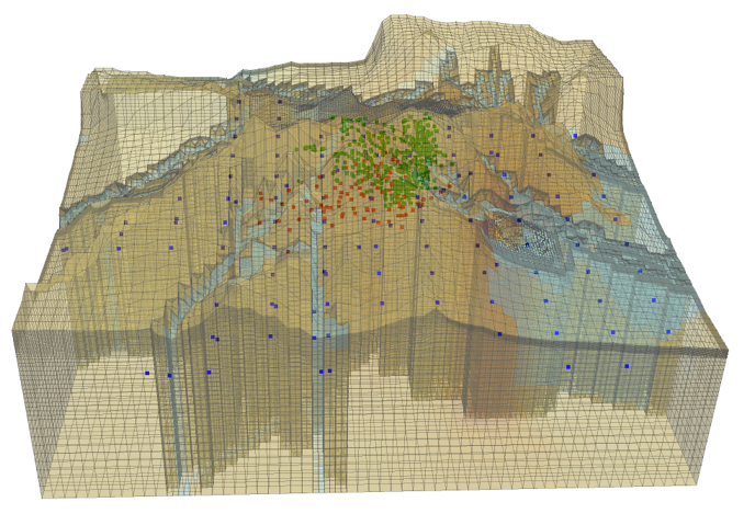
Pilot point parameterisation of a three-dimensional model domain and pervading structures.