Data space inversion (DSI) delivers the same outcomes as calibration and predictive uncertainty analysis without having to do either. It is stunningly model-run-efficient. What is more, it can be implemented with complex, slow-running models that are endowed with complex parameter fields whose prior probability distributions are difficult to characterise, and impossible to adjust.

Does this sound too good to be true?

It is indeed an amazing (and very simple) methodology.

DSI gains its computational efficiency by skipping model calibration. Virtually unlimited parameterisation complexity can be expressed, but no parameters are actually adjusted. Instead, DSI uses a complex model, endowed with realisations of complex parameter fields, to build a direct statistical relationship between the measured past and the managed future (the latter comprising predictions of management interest). Once these relationships are established, a "statistical model" can replace the groundwater model. This model runs extremely fast. It is this model that is subjected to Bayesian analysis. Once this has been done, it can (in theory) be used to make minimum a posteriori (i.e. MAP) predictions of future system behaviour. It can also associate prior and posterior uncertainties with these predictions.

Actually, it can do more than this.

Using the same workflow, you can build a statistical model that links fantasy measurements to the managed future. You can then determine which of these will be most effective in reducing the uncertainties of predictions that are important to you. This is somewhat similar to linear data worth analysis. However, because the analysis is nonlinear, it is more informative.

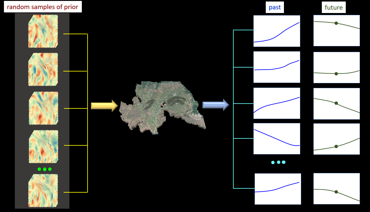
The following figure shows the first step in the DSI process. A model is run over the past and into the future using many different random parameter fields. (Often only a few hundred random realisations is fine.) The parameter fields can be of arbitrary complexity. They can embody different realisations from the same prior probability distribution, or they can embody realisations from different prior probability distributions. This allows you to express uncertainty in the prior. These parameter fields can also include categorical features such as faults. Perhaps these faults can be at different locations for different realisations. Nothing is off the table!

After having performed these model runs, it is an easy matter to select any future system state (one such state is shown in the above figure), and construct a histogram of that state. By doing this, you sample the prior probability distribution of that prediction.

This is nice. But our task is to sample the posterior probability distribution of the prediction.

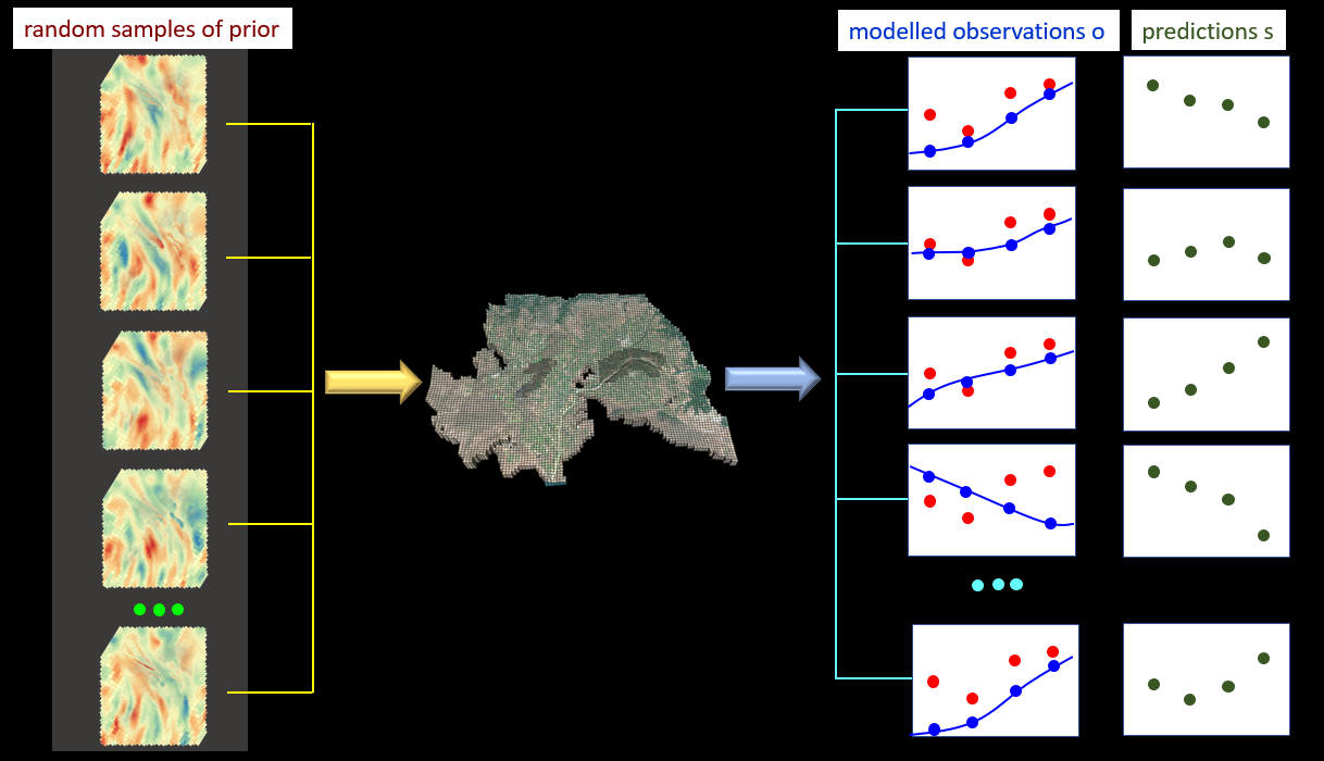
In the following figure the red dots represent field observations of system behaviour. The blue dots are the model-generated counterparts to these. We suppose that four predictions of management interest are required of the model. These are represented by the green dots.

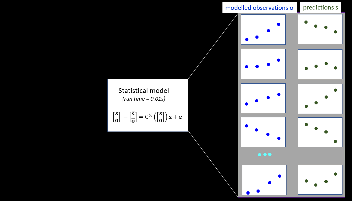
Now we put the model to one side. And for the moment we put field observations to one side too.

Using standard statistical formulas, we build a covariance matrix that links the measured past to the modelled future. (Actually there are a few tricks that can make this process more robust, such as histogram transformation. But we won't go into that.) This statistical model can be built in a few seconds using utilities supplied with PEST (see below).

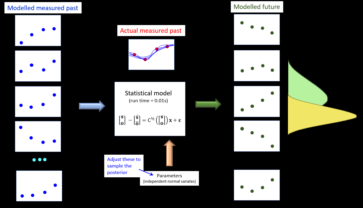
The statistical model is parameterised by elements of a vector x. The elements of x have independent normal prior probability distributions. If we history-match the statistical model against field measurements, we can determine the posterior probability distribution of x. We can then run the statistical model to determine the posterior probability distribution of predictions s.

How do we history-match the statistical model? In whatever way you like. PESTPP-IES is a handy option. History-matching is complete in a few seconds.

The entire process is schematised below.

The following table lists PEST-suite programs that can assist with data space inversion. See also programs that can be used for generation of stochastic fields of arbitrary complexity.