Analysis of uncertainty is itself uncertain.

In most geological circumstances that are the focus of groundwater modelling, we do not really know the prior probability distribution of model parameters. And even if, by some magic, we could capture the chaotic nature of the subsurface using some legitimate stochastic model, many numerical problems would beset calculation of a posterior probability distribution from this very complex prior.

The subsurface is full of surprises. Does the notion of "prior parameter probability distribution" even make sense?

In most cases of decision-support interest, we are really only interested in the pessimistic end of the posterior probability distribution of a decision-critical model prediction. This is the end where things go wrong. This is what can make or break a proposed management plan.

An alternative approach to assessing the possibility of something going wrong as a by-product of sampling the entire posterior probability distribution of a model prediction is to propose "something going wrong" as a hypothesis. According to the Popperian view of the scientific method, a scientific hypothesis can never be accepted; it can only be rejected. In the groundwater context, a "bad thing" hypothesis can be rejected if it is demonstrably incompatible with one or more of the following:

•processes that operate under the surface;

•the properties that govern these processes;

•the measured behaviour of the system.

Decision-support groundwater modelling, if properly conducted, is in a unique position to test a bad thing hypothesis against all three of these. Processes are encapsulated in a simulator's equations; hydraulic properties are encapsulated in its parameters; compatibility (or lack thereof) with measurements of system state can be tested using software from the PEST or PEST++ suites.

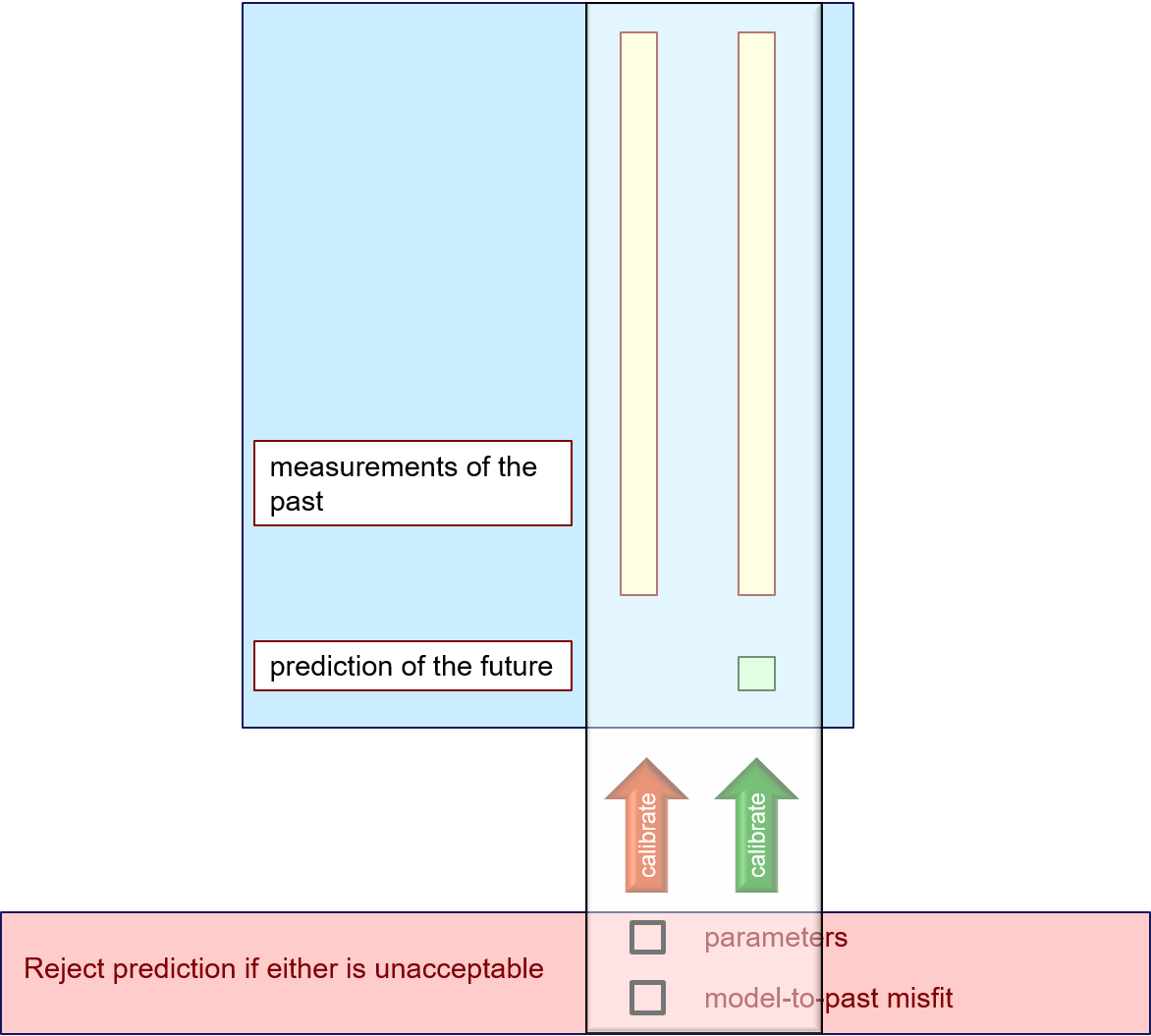
Suppose that we have just calibrated a groundwater model. What have we learned?

If we have done our regularisation properly, we have learned the minimum amount of hydraulic property complexity that is required for the model to replicate field measurements. We have also learned about the level of model-to-measurement misfit that we can expect for our model; this will often far exceed measurement noise. The first of these may have told us something about the prior probability distribution of model parameters that we did not previously know. The second of these has told us something about the likelihood function. These are the two terms of Bayes equation. Bayes equation (or the spirit of Bayes equation) is the path to exploration of posterior uncertainty.

But let's be practical. (When engaged in decision-support groundwater modelling, we have no other option but to be practical.)

Sometimes parameter fields that emerge from model calibration suggest that parameters are compensating for model defects. Ideally, we should try to prevent this behaviour by repairing the model. But we can never entirely eliminate it. Furthermore, for some predictions (particular data-driven predictions that are sensitive to solution-space components of model parameter space) weird parameters do not lead to weird predictions. So in learning about minimum required parameter heterogeneity from the model calibration process, we may learn that some parameters can, and should, adopt compensatory roles. At the same time, we learn what prior probability distribution we should bestow on them in order to accommodate this behaviour. (Or, more qualitatively, what level of parameter heterogeneity we can tolerate.)

Toleration of a certain level of model-to-measurement misfit is another way of accommodating model defects (in addition to tolerating a parameter-compensatory prior). The difference is that model-to-measurement misfit renders these defects visible, in contrast to defects that are hidden by compensatory parameter behaviour and therefore remain invisible. However it is difficult (if not impossible) to ascribe a statistical probability distribution to structural misfit. It follows that we cannot precisely define a likelihood function.

So what we learn from model calibration is generally qualitative. But this does not diminish its importance. What we learn from calibration are the standards by which predictive hypotheses can be scientifically tested.

The predictive hypothesis-testing workflow proceeds as follows.

1.Calibrate a model against a measurement dataset.

2.Now calibrate the model again. Include in the calibration dataset an unwanted value of a management-salient prediction.

3.If PEST can fit the unwanted prediction without incurring "intolerable" misfit with field measurements, or without introducing "intolerable" values to parameters (or patterns of parameters), then the hypothesis embodied in the prediction cannot be rejected.

"Intolerable" is a qualitative metric. However, much has been learned about "qualitative" from the previous calibration process.

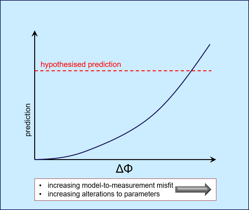
Direct predictive hypothesis-testing can sometimes be facilitated by running PEST in "Pareto" mode.

First, calibrate the model against the measured past. Then insert the calibrated parameters into a new PEST control file as initial parameters. (This PEST control file must tell the model to run into the future as well as over the past.) Add prior information equations that specify that initial parameter values are preferred parameter values (use ADDREG1 or ADDREG2). However PEST cannot run in "regularisation" mode and "Pareto" mode at the same time. So you must determine the appropriate regularisation weight factor yourself for prior information equations that specify minimal departure of parameters from their initial (i.e.calibrated) values.

One option is to use the final regularisation weights that PEST used in the previous calibration exercise. These can be obtained from the residuals file (i.e. the RES file) that PEST wrote at the end of that exercise. Alternatively, adopt the following strategy.

1.Use the PWTADJ2 utility to ensure that measurement weights are "correct", given the measurement objective function that was attained during model calibration. (The measurement objective function should then equal the number of observations.)

2.Set regularisation weights and covariances in accordance with your concept of the prior parameter probability distribution.

Add a "Pareto" section to the PEST control file and set PESTMODE to "pareto". Provide a value for the hypothesised prediction, an upper limit on its weight, and a weight increment. Then run PEST.

See the PEST manual for further details.

When run in "Pareto" mode, PEST slowly increases the weight on the prediction. If things work well, you then get to trade off respect for the past (and parameters that are calibrated against the past) against respect for the hypothesised future. Ideally, you can choose the point where the two are incompatible, and hence the value of the hypothesised prediction at which this prediction can be rejected.

There are two components of the objective function to inspect as the weight on the prediction increases. The first is that which characterises model-to-measurement misfit, while the second is that which characterises departures of parameters from their calibrated values. In the end, you will probably need to plot maps of parameters, and graphs of model outputs, in order to properly make a subjective call on what you are prepared to tolerate.