Calculation of predictive uncertainty under the assumptions of model linearity and Gaussian probability distributions is not too different from calculation of parameter uncertainty under these same assumptions. However we need one more ingredient. We need the sensitivity of a prediction of interest to all model parameters. If these comprise the elements of a vector y, we can say:

s = yTk

where s (a scalar) is the prediction of interest. (As usual, the "T" superscript denotes the transpose operator.)

From the above equation, the prior uncertainty variance of prediction s is easily formulated as:

σ2s = yTC(k)y

where C(k) is the prior covariance matrix of k.

The posterior covariance matrix of prediction s can be calculated using either of the following (mathematically equivalent) equations. (We use the prime superscript to distinguish posterior from prior.)

σ'2s = yT[JTC-1(ε)J + C-1(k)]-1y

σ'2s = yTC(k)y - yTC(k)JT[JC(k)JT + C(ε)]-1JC(k)y

The second of these equations in particular shows how uncertainty is reduced through history-matching (the Jacobian matrix J appears only in the second term). It is important to realise that history-matching may reduce the uncertainty of some predictions much more than that of others. This depends on the parameters to which predictions are sensitive, and on the parameters that measurements of historical system behaviour inform. If the parameters (or combinations of parameters) which govern the future behaviour of a system are very different from those which governed its past behaviour, the past may not have too much to say about the future.

Another page describes how you can obtain most of the matrices that appear in the above equations. We now turn our attention to how the y vector is obtained.

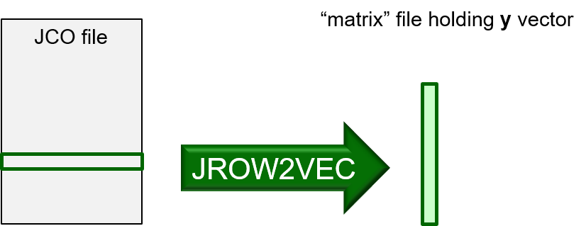
For some predictions, there is no need to run a model into the future in order to obtain its sensitivities to model parameters.

Suppose that we are calibrating a model against heads, and that we would like to use this same model to investigate something that has not been measured in the field, for example exchange of water with a stream, or the paths of agricultural contaminants. In this case, predictions of interest can be calculated by the same model that is being calibrated. Predictions can be read from model output files by PEST as if they are observations. Therefore, they are featured in a PEST control file. Predictions should be given weights of zero in this file so that they do not influence the parameter estimation process. Because they appear in a PEST control file, their sensitivities are recorded in the Jacobian matrix file that PEST writes as the model is calibrated.

In most circumstances however, predictions of interest occur in the future.

Calculation of future predictive sensitivities requires that the model be configured to run into the future, probably under a different stress regime from that which prevailed in the past. Furthermore, the model must be run by PEST as if it were being calibrated against predictions of interest. PEST setup should include all parameters that were estimated when the model was actually calibrated. Initial parameter values that are recorded in the "parameter data" section of the PEST control file should be values obtained through calibration. Instruction files must be created to read predictions of interest from model output files. The values that are assigned to these "predictive observations" in the PEST control file are immaterial, as PEST should not be asked to adjust parameters. It should be run with NOPTMAX set to -1 or -2 so that it calculates a predictive Jacobian matrix and then ceases execution.

Regardless of how they are calculated, sensitivities of a prediction of interest to model parameters can be extracted from a Jacobian matrix file using the JROW2VEC utility. That is, JROW2VEC produces the y vector that appears in the above equations.

The PREDUNC1 utility calculates the prior and posterior uncertainties of a prediction using equations that are presented above. It reads the following files:

•a PEST control file;

•a corresponding Jacobian matrix file;

•a parameter uncertainty file;

•a predictive sensitivity file.

To avoid confusion, weights should be "correct" in the PEST control file that PREDUNC1 reads. This is easily accomplished using the PWTADJ2 utility.

PREDUNC1 writes prior and posterior predictive uncertainties to the screen. PREDUNC6 is very similar to PREDUNC1. However it calculates the uncertainties of multiple predictions and records them in a file.

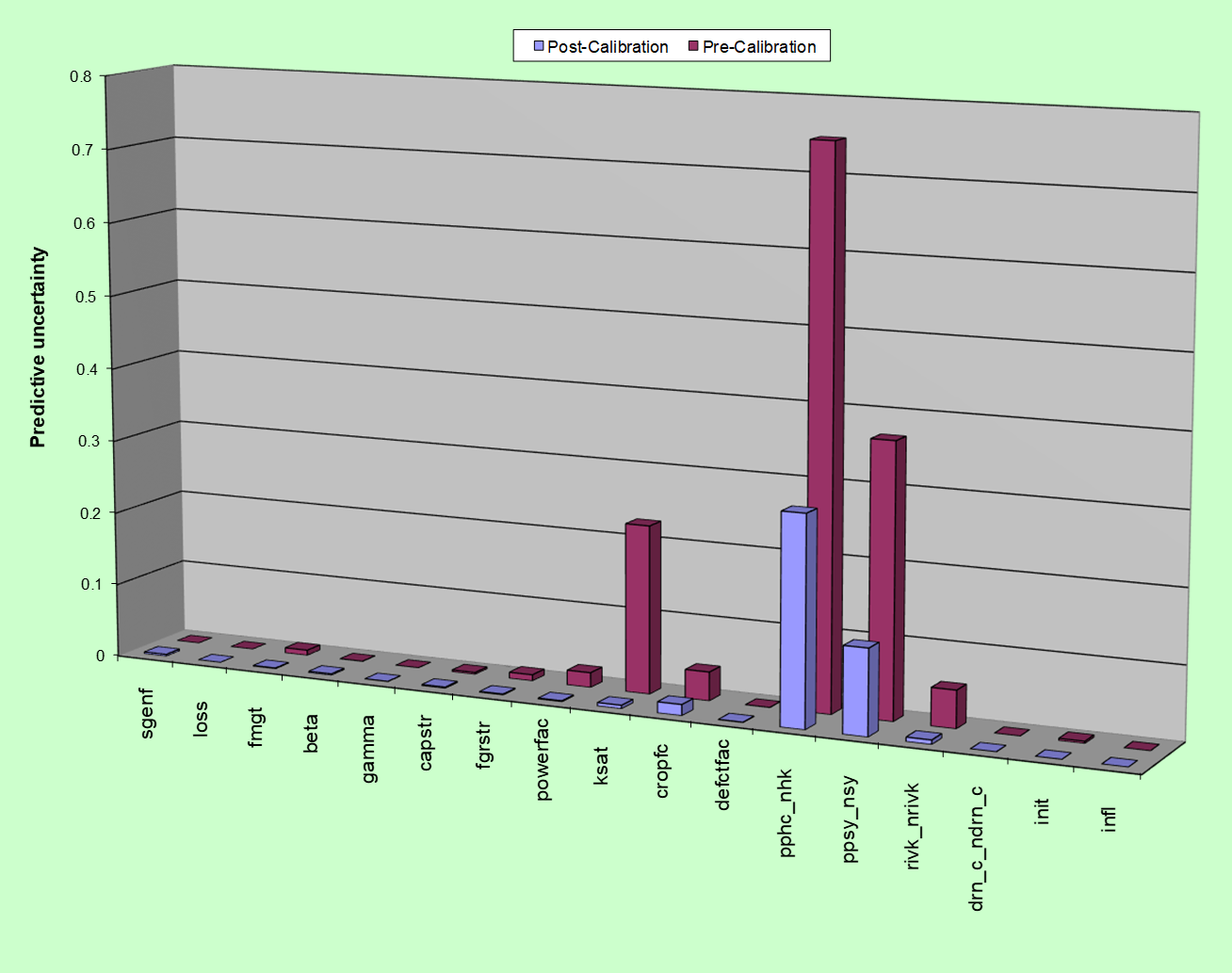
Definition

The equations that are presented above can be used to calculate the contribution that an individual parameter, or a group of parameters, makes to the uncertainty of a prediction of interest. We define "contribution to uncertainty" as the reduction in predictive uncertainty that would be accrued through attainment of perfect knowledge of the value of that parameter, or of the values of all parameters that comprise the group. This can be calculated for both prior and posterior uncertainties using the PREDUNC4 utility.

Contributions to the uncertainty of a groundwater level prediction by different parameter groups.

Some uses

Parameter contributions to uncertainty can reveal a lot about the nature of decision-support modelling as it pertains to a particular management issue.

The builder of a decision-support model is always faced with the problem of determining an appropriate level of complexity for his/her model. Simpler models are easier to build, run faster, and are numerically more stable than complex models. It is therefore easy for them to harvest information from data and quantify predictive uncertainty. However, simplification may induce predictive bias, either through construction or history-matching.

A simplified model is simple because it represents certain environmental processes and properties in an abstract manner. For example, it may replace part of an environmental system with a boundary condition. Parameters can be associated with simplifications and abstractions such as these. If the contributions that are made to decision-critical model predictions by these particular "simplification parameters" are small compared with those of other parameters, this suggests that model simplification has done little to harm the decision-support integrity of the model.

A paradox

Sometimes the contribution that a parameter or parameter group makes to the posterior uncertainty of a prediction is greater than its contribution to the prior uncertainty of the same prediction.

At first sight, this does not make sense. But it is easily explained.

Recall the definition of "contribution to uncertainty". This measures the reduction in predictive uncertainty accrued through acquisition of perfect knowledge of pertinent parameter values.

Suppose that two different parameters exhibit no prior correlation. The uncertainty of one of these parameters is therefore independent of that of the other. Suppose that a prediction of interest is sensitive only to the first parameter. The prior contribution of the second parameter to the uncertainty of this prediction is obviously zero.

Suppose now that the two parameters exhibit post-calibration correlation. This means that the information content of the calibration dataset is not enough to inform each parameter individually; it informs some linear combination of these two parameters (for example differences or sums of parameter values). It follows, therefore, that if the value of the second parameter becomes known, information that is resident in the calibration dataset can totally inform the first parameter. This is the parameter to which the prediction of interest is sensitive.

This is why the "contribution to the uncertainty" of the prediction that is made by the second parameter rises from nothing to something once history-matching constraints are imposed on parameter values.

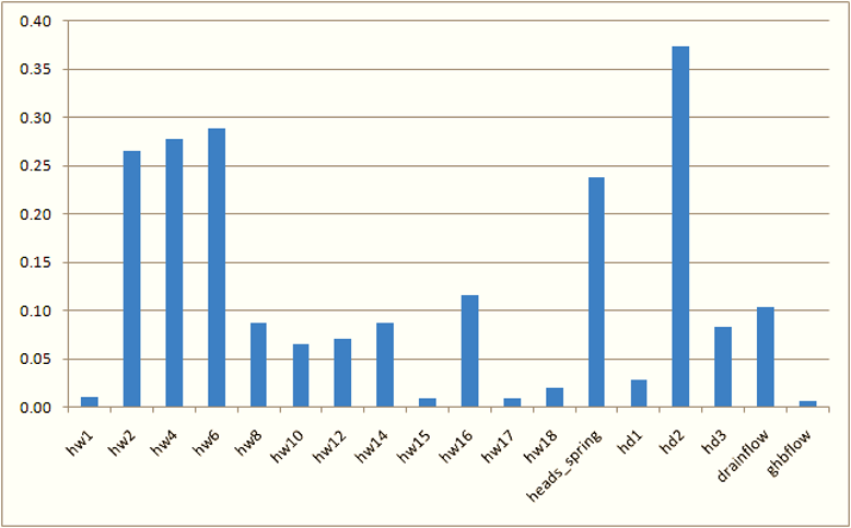
What is the worth of data?

The worth of data increase in proportion to their ability to reduce the uncertainties of predictions of management interest.

If we can quantify uncertainty, then we can quantify reduction in uncertainty. Therefore we can quantify data worth. This is particularly easy (though approximate) when uncertainty analysis is linear. This is because a fundamental premise of linear analysis is that sensitivities of prediction-pertinent and calibration-pertinent model outputs to model parameters are independent of the values of parameters. As a direct consequence of this, the matrix equations that are used to calculate prior and posterior predictive uncertainty feature the values of neither parameters, observations nor predictions. This means that we can use them to assess the revised uncertainty of a prediction of interest on acquisition of new measurements without having to know the values of these measurements!

Data worth analysis can be implemented manually through repeated use of PREDUNC1 or PREDUNC6. However the PREDUNC5 utility automates the process. The worth of individual measurements, or of a whole measurement type (e.g. heads or concentrations) can be readily evaluated.

The following figure demonstrates the worth of components of an existing calibration dataset by displaying the extent to which the uncertainty of a prediction of management interest would rise if each component were omitted from it.  

Increase in uncertainty of a prediction incurred through loss of different types of data from the calibration dataset.