In a sense, all ensemble methods are pseudo-linear, as their theory is based on linearity of model outputs with respect to parameters. However their speed, ease of use, ability to accommodate stunningly large numbers of parameters, and the approximate nature of simulation itself, makes their use attractive.

For a while now, the PEST suite has offered alternative methods of posterior uncertainty analysis which also have their roots in linear theory. With the advent of programs such as PESTPP-IES, these are not used as much now. Their use requires that a model first be calibrated, and that a Jacobian matrix then be calculated. This reduces the number of parameters that can be featured in the analysis.

Nevertheless, there are still occasions where these methods may prove useful. These are data-rich, nonlinear contexts where the integrity of uncertainty intervals calculated using ensemble methods may be challenged by limitations in their ability to probe the parameter null space in a bias-free manner.

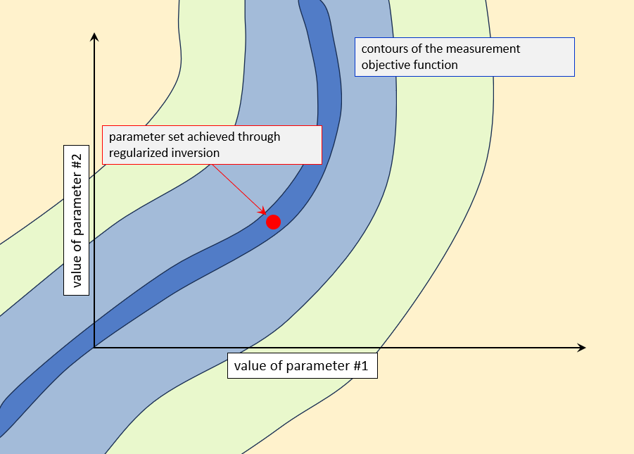
First calibrate the model. This brings with it certain benefits. It allows a modeller to test the current hydrogeological conceptual model. This testing may expose processes and/or important aspects of subsurface hydraulic property heterogeneity of which a modeller was previously unaware. This, in turn, may help him/her to formulate a more appropriate prior parameter probability distribution than that which had been previously adopted for the site.

The situation is depicted in the following picture - vastly simplified because we consider only two parameters (in order to have a picture). Notice that objective function contours do not close as the inverse problem is ill-posed. The "minimum" of the objective function is in fact a long valley (shown in blue).

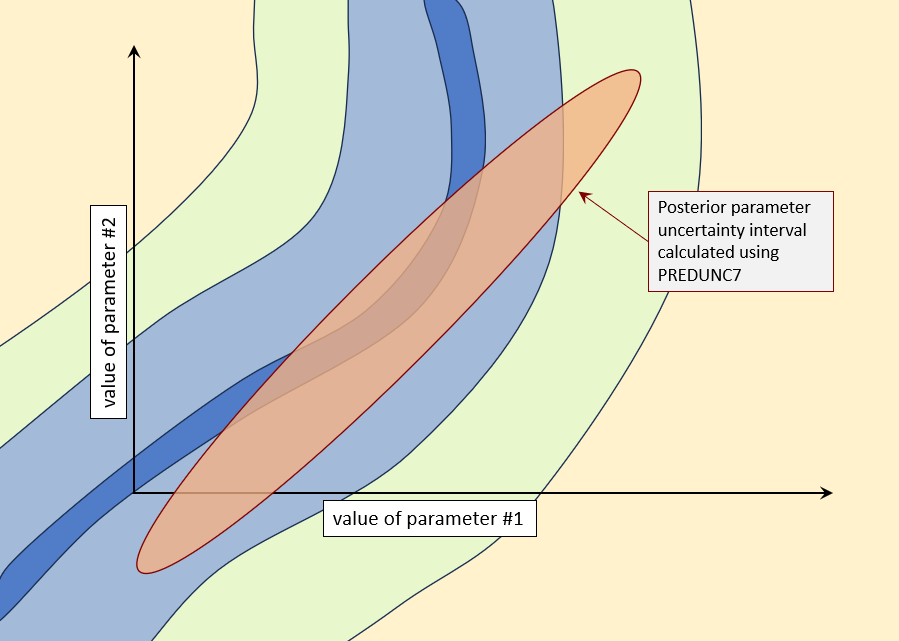
Next create a new PEST control file in which calibrated parameters feature as initial parameters. Calculate a Jacobian matrix. Then use linear analysis utilities supplied with PEST (particularly the PREDUNC7 utility) to calculate a posterior parameter covariance matrix. See the picture below. The elliptical parameter uncertainty contour reflects the assumption of model linearity.

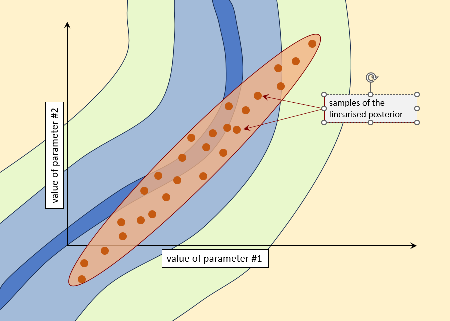
Now sample the linearised posterior parameter probability distribution using programs of the RANDPAR family. See below.

There are a few options of what to do next.

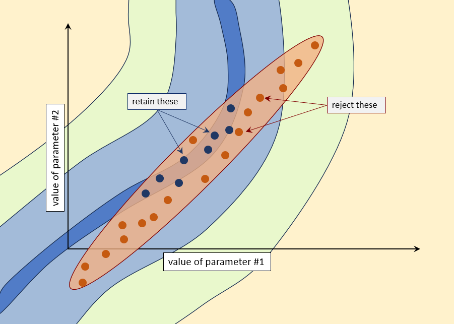
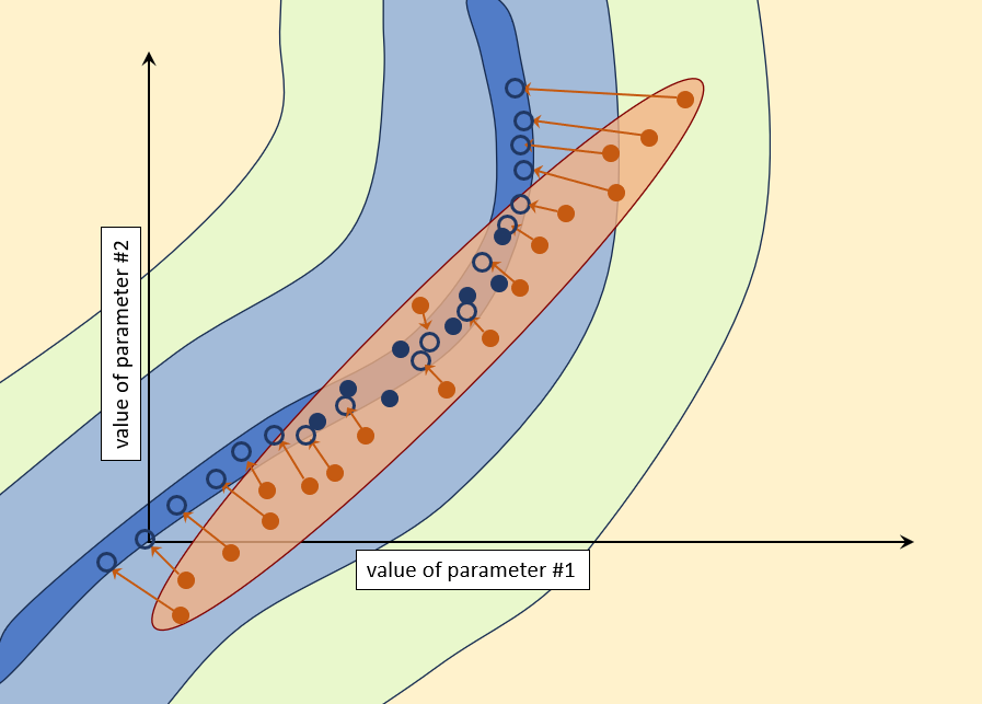
The easiest option is to throw away parameter samples for which the measurement objective function is above a certain value. Then, when you make a model prediction of management interest, use only those samples that allow the model to replicate the past (to the extent that you deem adequate). This option is depicted below.

This strategy has the advantage of simplicity. And it may be a good option where most of the samples of the linearised posterior allow the model to fit field measurements well. However in other circumstances too many samples may be rejected. There is also a risk that posterior predictive uncertainties may be underestimated.

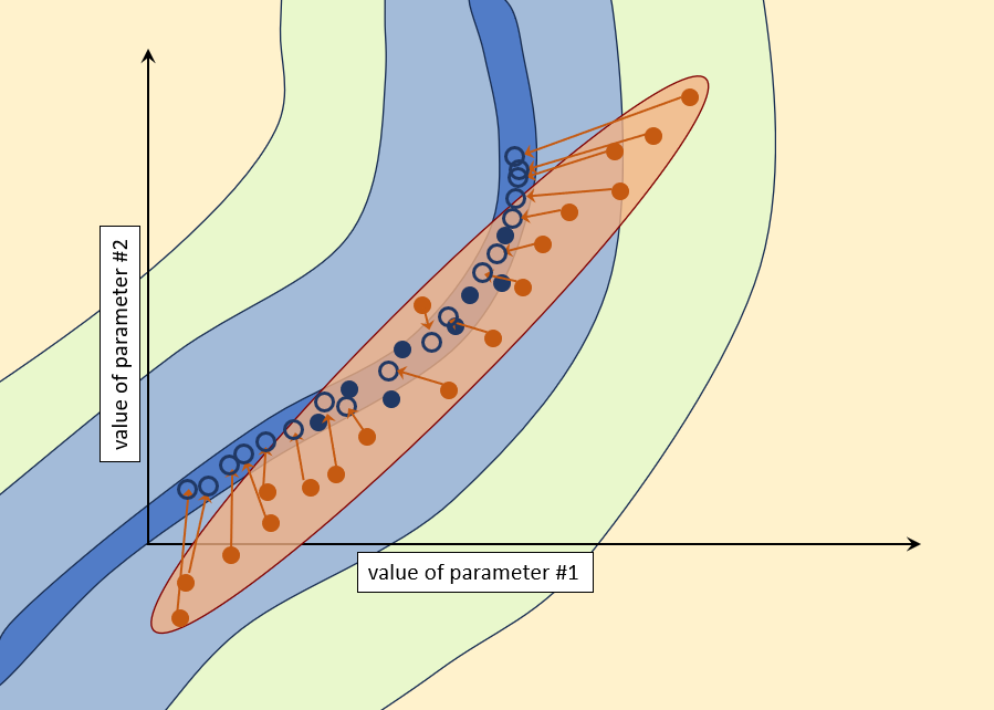
A second option is to adjust all the non-conforming parameter sets until they conform. This can be done using PEST. Furthermore, to preserve diversity of parameter sets, Tikhonov regularisation can be introduced to the parameter adjustment process so that each adjusted random parameter set moves the minimum distance in parameter space that is required for the model to replicate field measurements. This may sound a little complicated. However the process is easily automated. Use the PARREP and ADDREG2 utilities to construct the PEST control file that underpins each inversion process. Include the repetitive adjustment process in a batch or script loop.

Now you may be thinking that this is going to be a VERY model-run-intensive procedure. Actually no.

Don't forget that you calculated a Jacobian matrix before running PREDUNC7 to obtain the linearised posterior covariance matrix. Well, if you start PEST with the "/i" switch, it will use this Jacobian matrix for the first iteration of the inversion process instead of calculating a new Jacobian matrix using finite parameter differences. So the first iteration of the random parameter adjustment process is virtually free for all parameter sets. (Some parameter sets may not actually require adjustment at all.) Perhaps most parameter sets will require no more than one iteration of adjustment. Or perhaps you can decide that you will reject parameter sets that require more than one iteration of adjustment because they are too far away from the valley of objective function minima.

The process is schematised below.

This option is easy. Simply bypass the use of ADDREG2. Omission of Tikhonov regularisation from the parameter adjustment process renders individual parameter sets far more amenable to adjustment. A far greater number of random parameter sets may therefore achieve a suitably low measurement objective function after just one iteration of adjustment. Recall that this iteration comes for free.

This may be a good thing; or it may be a bad thing. Lack of random-parameter-set-specific regularisation may work against parameter set diversity. However, if a greater number of parameter sets can be quickly adjusted to the point where the measurement objective function is suitably low, then this may actually promote parameter set diversity.

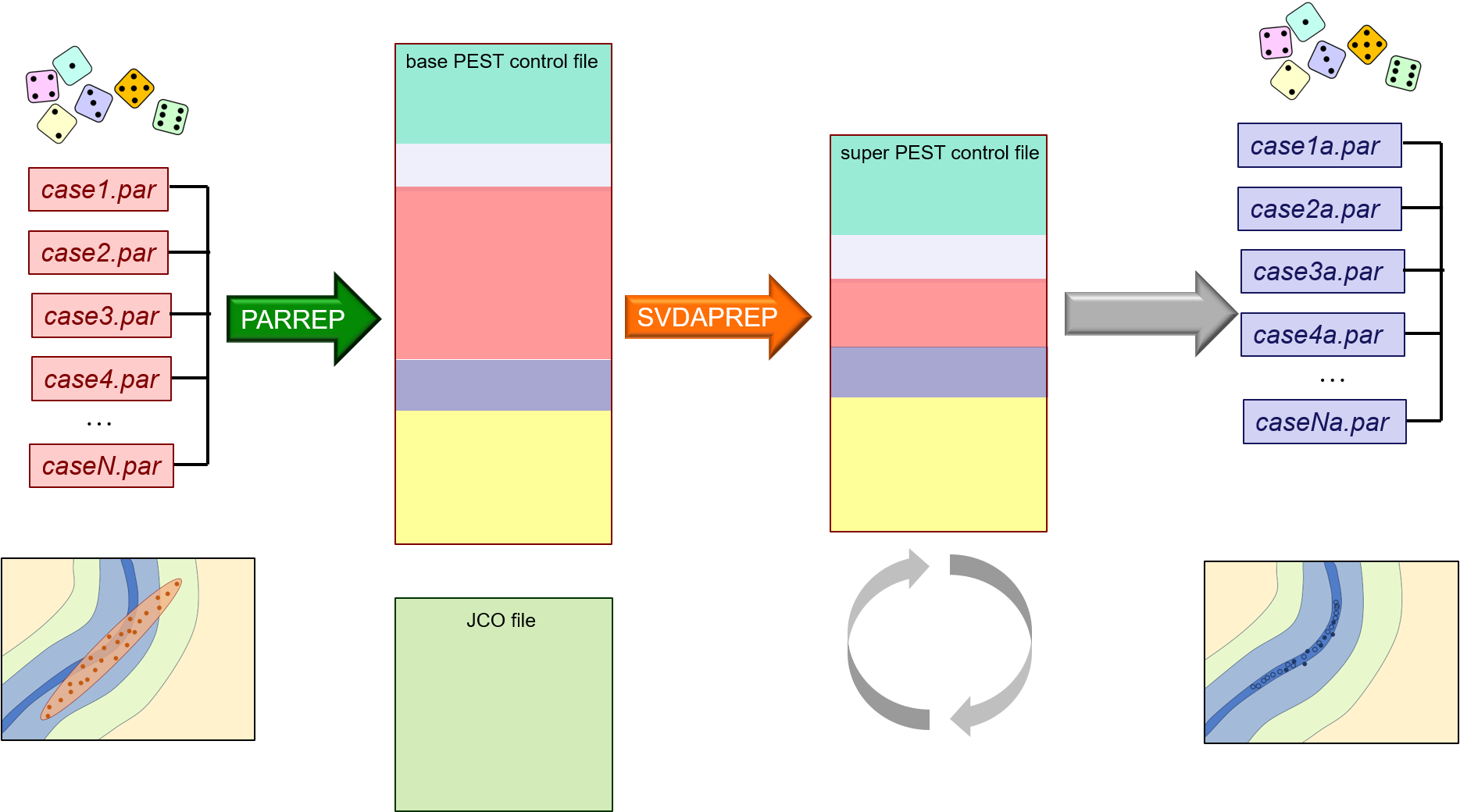
If it turns out that parameters will require a second iteration of adjustment, then you may as well do this cheaply. So use SVD-assist to undertake repetitive adjustment of random parameter sets. (Don't forget that when you undertake SVD-assisted inversion, the first iteration of the inversion process is nearly model-run free; so only the second iteration requires many model runs. However it requires only as many model runs as there are super-parameters, not native model parameters.)

This method is referred to as "null space Monte Carlo".

The workflow is simple.

Using the SVDAPREP utility, build a PEST control file that is set up for SVD-assisted inversion. Don't forget that you already have a Jacobian matrix for the base parameter PEST control file; you needed this to run PREDUNC7 in order to calculate the linearised posterior covariance matrix. Also, setup for SVD-assisted inversion is easier if you don't undertake regularisation that is specific to each random parameter set; so this is an extension of option 3.

You can set up a batch loop so that repetitive adjustment of many parameter sets is automated. (This is explained in the PEST manual.) Use the PARREP utility to insert each random parameter set into the base PEST control file. Then run PEST on the super-parameter PEST control file. Tell PEST to stop after two iterations. The first iteration is virtually free (and may be enough to attain a good fit with the history-matching dataset). The second is cheap.

Null space Monte Carlo.

The PNULPAR utility (supplied with PEST) can be used instead of PREDUNC7 to support sampling of the linearised approximation to the posterior parameter probability distribution. It can also be used following PREDUNC7, so that you use the two together. PNULPAR works by projecting parameter fields onto the calibration solution space. The smaller that you inform PNULPAR is the dimensionality of the solution space, the better will samples of the linearised approximation to the posterior parameter probability distribution fit the measurement dataset. The less adjustment will they therefore require.

The outcome of the repetitive history-matching process that is described above is a series of parameter value files (i.e. PAR files - or BPA files if using SVD-assist). These files contain samples of the posterior parameter probability distribution. To sample the posterior probability distribution of predictions of management interest, run the model into the future using these parameter sets.

The easiest way to accomplish this is to modify the PEST control file that was used for history-matching so that it runs the predictive model rather than the history-matching model. Set the NOPTMAX control variable to 0 in this PEST control file, and then use the PARREP utility to insert the contents of posterior PAR or BPA files into the PEST control file. This process is easily automated. Declare predictions of interest to be observations in this PEST control file. Their "observed values" and weights do not matter.

The following table lists program from the PEST suite that can help with workflows that are described above. Many of these utilities are discussed in other pages. See also programs that are used for model run postprocessing in general.