This page provides a brief overview of what comprises the PEST suite. Other pages discuss the software that is listed below in greater detail, while describing workflows in which they play an indispensable part. All of these programs can be downloaded from the PEST web pages.

If you download PEST you receive over 200 programs. A brief overview of these programs follows. (Do not be daunted. Some programs of the PEST suite are a little old now, but are still included in the suite as some people may find them useful. These web pages will make it clear which programs of the PEST suite are right for you.)

PEST itself

PEST undertakes regularised or unregularised inversion (i.e. calibration). In doing this, it runs a model many times, all the while upgrading its parameters until a good fit is attained between model outputs and field measurements. Its algorithms are sophisticated and flexible. They can tolerate bad numerical model behaviour. They can even use different versions of the same model for different inversion subtasks.

There are other things that PEST can do as well. When run in "predictive analysis" mode, PEST can maximise a model prediction subject to the constraint that the model stays calibrated.  It can undertake model runs that convey it smoothly across a two-dimensional Pareto front. Or it can simply undertake a bunch of model runs and record the outcomes of these runs for later analysis.

BEOPEST does the same things that PEST does. However model runs can be conducted in parallel, either on the same or on different computers (or in the cloud).

Setup utilities

Many of the programs that are supplied with PEST automate construction and/or modification of part or all of its input dataset. These facilitate PEST setup for specific tasks.

Linear sensitivity and uncertainty analysis

The inversion algorithm that is implemented by PEST requires that it calculates a sensitivity matrix (also known as a Jacobian matrix). Some of PEST's utility support programs allow you to view part or all of this matrix, and optionally modify it in ways that can increase your understanding of the inversion process. Other utilities support first order second moment (FOSM) analysis of prior/posterior parameter/predictive uncertainty. Ancillary analyses such as worth of existing or contemplated data (with "worth" of data increasing in proportion to their ability to reduce uncertainty) can also be performed.

Problem diagnosis

PEST doesn't always work. Is this because of PEST? Is it because of the model? Is it because of some feature of the inverse problem? Utility programs that are supplied with PEST can explore these issues. The information that they provide can be really useful, whether or not you use PEST.

Matrix manipulation

When undertaking history-matching and uncertainty analysis, you encounter matrices everywhere - especially Jacobian matrices and covariance matrices. Utilities provided with PEST allows you to manipulate, combine and multiply these matrices. You can also perform more complicated tasks such as singular value decomposition.

Data space inversion

Data space inversion (DSI) is a relatively new technology that supports innovative and insightful ways of using models in decision support. Start the process by running a model only a few hundred times using stochastic parameter fields of arbitrary complexity. Then use software supplied with PEST to construct direct statistical linkages between the measured past and the managed future. These can be encapsulated in a surrogate model that is effortlessly history-matched using PEST or PEST++. Predictions of future system behaviour are thereby data-informed; their uncertainties are quantified.

Global Optimisation

Where model behaviour is messy and nonlinear (either because of deficiencies in the model's numerical algorithm, or because of system complexities), then local optima may make history-matching difficult. The CMAES_P and SCEUA_P global optimisers can work in this difficult modelling terrain - but only if model run times are relatively short. (This is always a problem with global optimisers).

"HP stands for "high performance" or "highly-parallelised". You can choose.

PEST_HP

PEST_HP is an improved version of BEOPEST. It dispenses with some aspects of PEST functionality (such as constrained prediction maximisation/minimisation) in order to concentrate on others. Its inversion engine is more powerful than that of PEST, and also more robust. Its efficient "randomised Jacobian" functionality can reduce model run times enormously in very highly parameterised contexts. Other efficiencies can be gained through simultaneous parameter increments and Jacobian matrix blanking. Parameterisation flexibility is offered through the use of secondary parameters.

PEST_HP comes with a program named PWHISP_HP. This is the "PEST whisperer". After the cessation of PEST_HP execution, the whisperer reads a suite of its output files. It provides advice on settings that may improve its performance.

CMAES_HP

CMAES_HP is a parallelised version of the CMAES_P global optimiser supplied with PEST. Use of "file parameters" supports basic optimisation under uncertainty. (There are quite a few articles in the groundwater literature on use of CMAES in wellfield optimisation.)

RSI_HP

RSI stands for "realisation space inversion". This is a kind of iterative ensemble smoother. RSI is fast and efficient in highly nonlinear settings. However it does not provide all of the functionality that is provided by PESTPP-IES. In particular, the cost of its fast convergence is a lack of ability to perform localisation.

PLPROC stands for "parameter list processor". PLPROC is a parameterisation engine that is used as a simulator preprocessor when a model is undergoing history-matching. It supports all combinations of the following parameterisation types with models that use both structured and unstructured grids.

•zone-based parameterisation

•pilot points (2D, 3D and linear along polylinear features of arbitrary complexity)

•spatial interpolation from pilot points to an arbitrary grid using kriging, radial basis functions and inverse power of distance

•spatially varying anisotropy

•alluvial channel parameterisation

•polylinear and polygonal structural overlay parameters with history-match-adjustable shapes

•variogram hyperpararameters

•linear and nonlinear, spatially varying relationships between parameters of the same or different types

Structural overlay parameters representing faults penetrate 20 out of 21 layers of a 3D model that explores inflow to a tunnel.

Like PEST, PLPROC communicates with a model through the model's own input and output files.

OLPROC stands for observation list processor". OLPROC runs after a simulator when a model is undergoing history-matching. It undertakes temporal interpolation of model outputs to the times at which field measurements were made. It can formulate secondary model outputs/observations from primary model outputs/observations. It writes output files that PEST can read, and instructions that teach PEST how to read them. It calculates weights to assign to different observations and observation types. Equations of arbitrary complexity can be used in weights formulation.

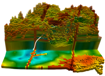
The Groundwater Utility suite is comprised of over 170 programs. Some of these have been superceded by programs such as PLPROC and OLPROC. Others provide functionality that can be found nowhere else. The groundwater utility suite is under constant development.

Roles performed by different members of this suite include the following:

•zonal and pilot point parameterisation

•construction of 2D and 3D spatial covariance matrices used for pilot point regularisation and uncertainty analysis based on stationary and nonstationary variograms

•construction of cell-based 2D/3D stochastic fields based on stationary/nonstationary variograms for structured/unstructured grids

•spatial and temporal interpolation from structured/unstructured grids to sites at which measurements were made

•reading of MODFLOW, MODFLOW 6 and MODFLOW-USG binary dependent variable and budget files

•extraction of arrays from MODFLOW, MODFLOW 6 and MODFLOW-USG input files

•provision of a rudimentary interface between MODFLOW, MODFLOW6 and MODFLOW-USG models on the one hand and display/processing platforms such as SURFER, GRAPHER, PARAVIEW and GIS packages on the other hand

•automation of PEST input dataset construction for complex measurement datasets

A 3D stochastic hydraulic property field governed by a spatially varying covariance function.

These are a little old now, but are still useful.

Chief among them is TSPROC. TSPROC stands for "time series processor". Tasks which it performs include the following:

•reading of output files generated by a number of different surface water models

•interpolation to the times at which measurements were made

•volume accumulation over regular or irregular intervals

•low pass, high pass and baseflow filtering/extraction

•calculation of flow duration statistics

•incorporation of all of the above into a comprehensive calibration dataset

Note that an improved version of TSPROC is available at this USGS website.

TS6PROC is a time-series preprocessor for MODFLOW 6.

TS6PROC reads a MODFLOW 6 time series file. It manipulates time series that are contained in this file, and then writes a new MODFLOW 6 time series file that contains the altered time series. This altered file can be used by MODFLOW 6 in place of the original one. Parameters that govern processing of time series can be earmarked for calibration adjustment

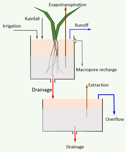
LUMPREM is a lumped-parameter recharge model. Two soil moisture stores calculate fast and slow recharge to a groundwater system.

Water is obtained from rainfall and lost to evapotranspiration and recharge. Water can also be obtained from irrigation on an as-needed basis. LUMPREM-calculated recharge time series can be formatted for use by a groundwater model. A LUMPREM postprocessor can write MODFLOW 6 time series file. Soil moisture store volumes can be transformed to simulate to provide time-varying boundary conditions for a groundwater model.

Design elements of the LUMPREM soil water balance model.

Some programs of the PEST suite come in multiple versions. An "_MKL" suffix to the program name indicates use of the MKL library. "MKL" stands for "math kernel library". Programs that are linked to this library can undertake large matrix operations such as singular value decomposition much faster than programs that are not linked to it. The speed difference is not so noticeable unless the problem size (generally linked to the number of parameters) is large. Where parameters number in the thousands, or in the tens of thousands, the difference in execution speed may be huge.